|
|
|
|
Continuous time-varying Q-factor estimation method in the time-frequency domain |
Although the CFS and LCFS methods assume that the amplitude spectrum
is Gaussian shape, they are still applicable to other spectra that fit
well to the Gaussian spectrum, such as the Ricker wavelet
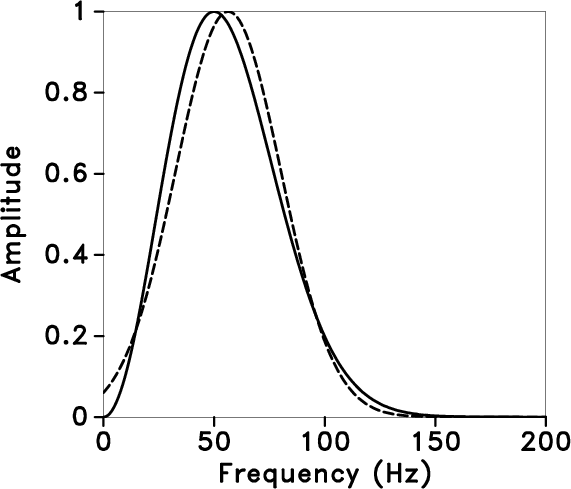
(Quan and Harris, 1997). The solid line in Figure 4 is the
amplitude spectrum of the Ricker wavelet (the dominant frequency is 50
Hz). According to the centroid frequency (![]() Hz) and variance
(
Hz) and variance
(
![]() ) of the amplitude spectrum, the Gaussian
spectrum can be synthesized (dotted line in
Figure 4). The two amplitude spectra can be well
fitted. In this paper, the Ricker wavelet is selected as the source
wavelet to verify the effectiveness of the LCFS method in estimating
the Q-factors. The Ricker wavelet with the dominant frequency of 50 Hz
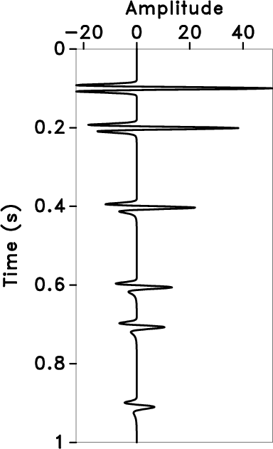
is used as the source wavelet to convolute with the reflectivity
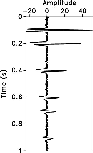
series to generate the attenuation model
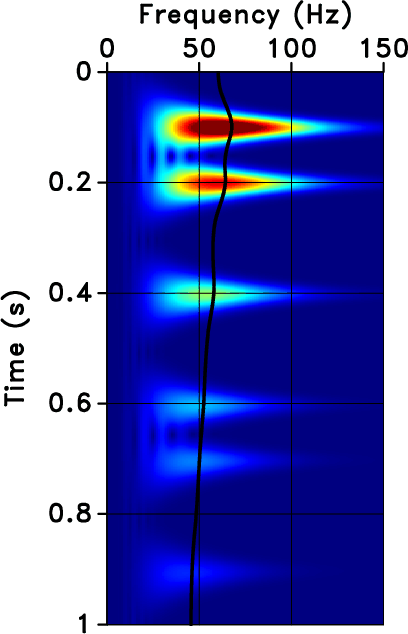
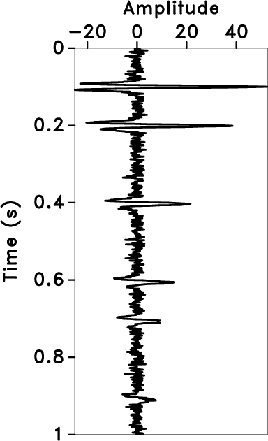
(Figure 5a). The time sampling interval is
1 ms, and the maximum propagation time is 1 s. There is one reflection
interface at 0.1, 0.2, 0.4, 0.6, 0.7, and 0.9 s respectively, and the
Q-factor of the formation is set to a constant value of 60, wherein
the first layer is set to be
unattenuated. Figure 5b shows the
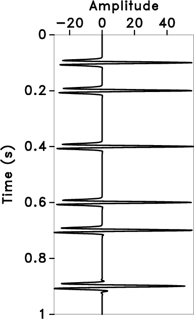
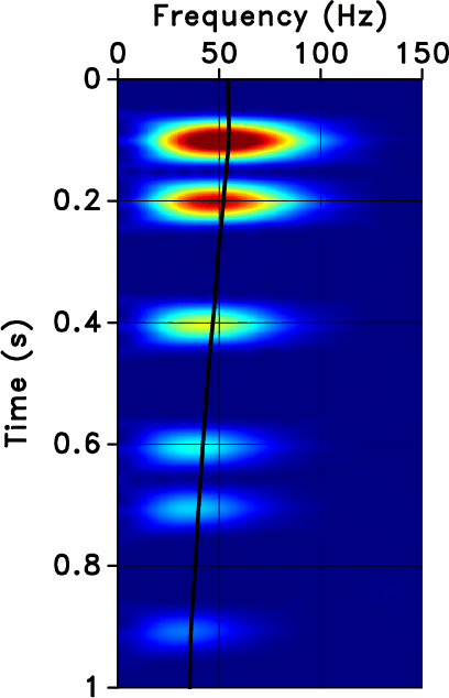
time-frequency spectrum of the attenuated signal obtained using the
LTFT method. The LTFT method can accurately represent the
time-frequency characteristics, wherein the black line is the local
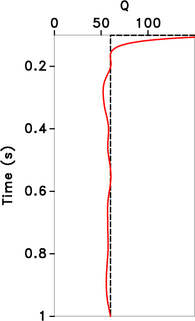
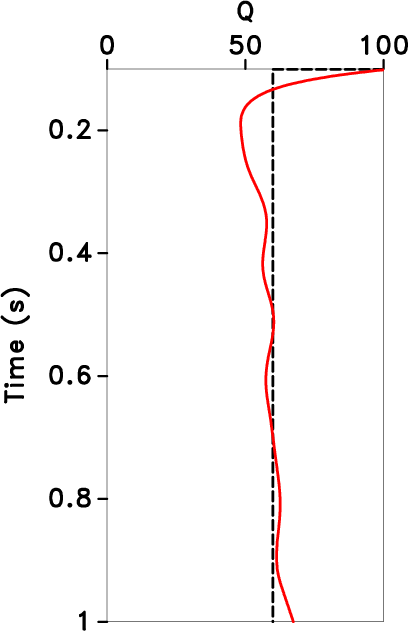
centroid frequency estimated using shaping regularization. By taking
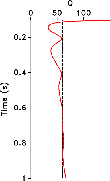
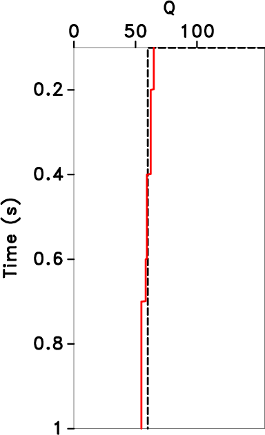
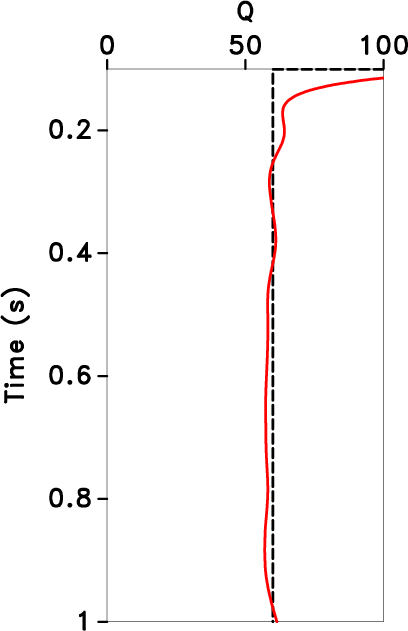
the local centroid frequency at 0.1 s as the referzence value, the
time-varying Q-value curve calculated using equation 19 is
shown as the red line in Figure 5c. The
black dotted line is the theoretical Q value. We can see that the
time-varying Q value estimated using the proposed method is close to
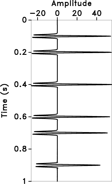
the theoretical Q value. Inverse Q filtering is performed using the
estimated time-varying Q-factors, and the result is shown in
Figure 5d. It can be seen that the
amplitude and phase of the wavelets are well recovered.
Figure 6 is the result estimated using the
proposed method in the S-transform
domain. Figure 6a is the time-frequency
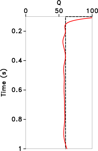
spectrum of the S-transform, and the black line is the local centroid
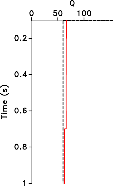
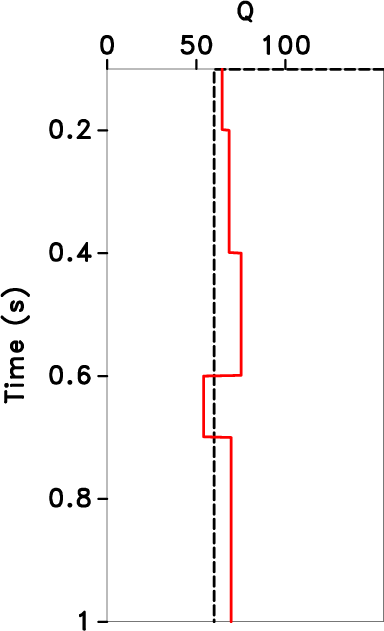
frequency. Figure 6b shows the time-varying Q
values estimated using the LCFS method, where the estimated result
before 0.6 s has a large error relative to the result estimated using
the LTFT method, and the estimated result after 0.6 s is close to the
theoretical one. Figure 6c shows the inverse Q
filtering result, and it can be seen that the amplitude and phase are
also reasonably recovered. According to the attenuation model test
with constant Q, we conclude that the LCFS method can also get
relatively accurate results at times without spectrum information, and
more reasonable results can be obtained using a reasonable
time-frequency transform.
) of the amplitude spectrum, the Gaussian
spectrum can be synthesized (dotted line in
Figure 4). The two amplitude spectra can be well
fitted. In this paper, the Ricker wavelet is selected as the source
wavelet to verify the effectiveness of the LCFS method in estimating
the Q-factors. The Ricker wavelet with the dominant frequency of 50 Hz
is used as the source wavelet to convolute with the reflectivity
series to generate the attenuation model
(Figure 5a). The time sampling interval is
1 ms, and the maximum propagation time is 1 s. There is one reflection
interface at 0.1, 0.2, 0.4, 0.6, 0.7, and 0.9 s respectively, and the
Q-factor of the formation is set to a constant value of 60, wherein
the first layer is set to be
unattenuated. Figure 5b shows the
time-frequency spectrum of the attenuated signal obtained using the
LTFT method. The LTFT method can accurately represent the
time-frequency characteristics, wherein the black line is the local
centroid frequency estimated using shaping regularization. By taking
the local centroid frequency at 0.1 s as the referzence value, the
time-varying Q-value curve calculated using equation 19 is
shown as the red line in Figure 5c. The
black dotted line is the theoretical Q value. We can see that the
time-varying Q value estimated using the proposed method is close to
the theoretical Q value. Inverse Q filtering is performed using the
estimated time-varying Q-factors, and the result is shown in
Figure 5d. It can be seen that the
amplitude and phase of the wavelets are well recovered.
Figure 6 is the result estimated using the
proposed method in the S-transform
domain. Figure 6a is the time-frequency
spectrum of the S-transform, and the black line is the local centroid
frequency. Figure 6b shows the time-varying Q
values estimated using the LCFS method, where the estimated result
before 0.6 s has a large error relative to the result estimated using
the LTFT method, and the estimated result after 0.6 s is close to the
theoretical one. Figure 6c shows the inverse Q
filtering result, and it can be seen that the amplitude and phase are
also reasonably recovered. According to the attenuation model test
with constant Q, we conclude that the LCFS method can also get
relatively accurate results at times without spectrum information, and
more reasonable results can be obtained using a reasonable
time-frequency transform.
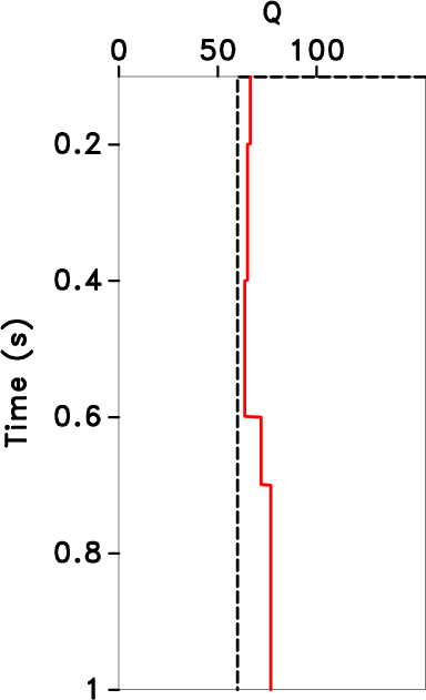
The traditional methods for estimating Q-factors in the time-frequency domain need to extract spectral information from the target layer’s top and bottom interfaces. In contrast, the method proposed in this paper only needs to extract information from a reference interface. We compare the proposed method with the traditional SR and CFS methods to further clarify its effect. We first extract the frequency spectrum of the corresponding time at the maximum amplitude of the six interfaces (extracted in Figure 5b) and estimate the Q-factors using the SR and CFS methods and interpolate them. The results are shown in the red lines in Figures 7a and 7b, respectively (the black dotted line represents the theoretical value). Then, we change the picking time and estimate the Q-factors using the SR (Figure 7c) and CFS (Figure 7d) methods. In Figure 7, we can see that the conventional Q-estimation methods need to pick the reflection interface accurately, but it is difficult to achieve in the actual seismic data processing.
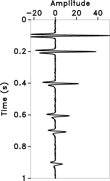
We estimated Q-factors in noise-added attenuated signals to confirm the stability and effectiveness of the LCFS method. Random noise of diff erent levels is added to the attenuated signal, as shown in Figures 8a, 8d, and 8g, respectively. The time-frequency distributions (Figures 8b, 8e, and 8h) of the noise-added signals are calculated using the LTFT method, wherein the black lines represent the local centroid frequencies. The red lines in Figures 8c, 8f, and 8i represent the time-varying Q-factors estimated using the proposed method. From the processing results of the noise-added signals, the LCFS method can also obtain relatively stable Q-factors in the presence of noise.
|
|---|
|
gau-ric
Figure 4. Amplitude spectrum of the Ricker wavelet (solid line) and the Gaussian spectrum (dotted line). |
|
|

|
|---|
|
asignal,fp,qq,cmsig
Figure 5. Attenuated model and estimated results. The attenuated model with constant Q (a), the time-frequency spectrum of the LTFT (the black line represents the local centroid frequency) (b), Q estimated using the LCFS method (red line) and theoretical Q (black dotted line) (c), inverse Q filtering result (d). |
|
|
|
|---|
|
fp1,qq1,cmsig1
Figure 6. Results estimated using the S-transform. The time-frequency spectrum of the S-transform (the black line represents the local centroid frequency) (a), Q estimated using the LCFS method (red line) and theoretical Q (black dotted line) (b), inverse Q filtering result (c). |
|
|
|
|---|
|
difsrq-1,difcfsq-1,difsrq-2,difcfsq-2
Figure 7. Estimated Q-factors using different methods (red line: estimated Q-factors; black dotted lines: theoretical Q-factors). The SR method (maximum amplitude) (a), CFS method (maximum amplitude) (b), SR method (nonmaximum amplitude) (c), CFS method (nonmaximum amplitude) (d). |
|
|


|
|---|
|
asignal,fp,qq,asignal1,fp1,qq1,asignal2,fp2,qq2
Figure 8. Noise-added attenuated signal and estimated results. The noise-added attenuated signal, and noise intensity increases gradually (a), (d), (g), the time-frequency spectrum of the LTFT (black lines represent the local centroid frequencies) (b), (e), (h), Q estimated using the LCFS method (red line) and theoretical Q (black dotted line) (c), (f), (i). |
|
|
|
|
|
|
Continuous time-varying Q-factor estimation method in the time-frequency domain |