|
|
|
|
Continuous time-varying Q-factor estimation method in the time-frequency domain |
To verify the feasibility of calculating the local centroid frequency
using the LTFT method, a nonstationary signal
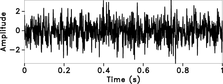
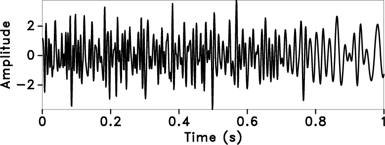
(Figure 1b) is generated by convolving the Ricker
wavelet with a random reflection coefficient
(Figure 1a). The dominant frequency of the signal is a
function varying with time
![]() .
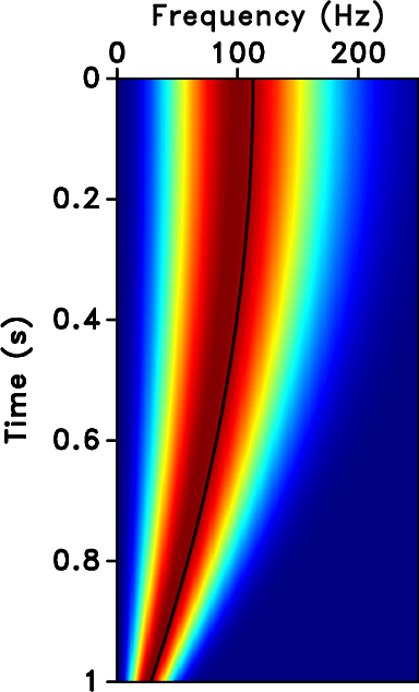
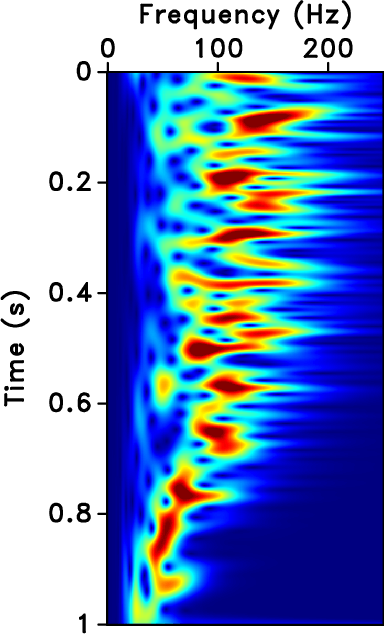
Figure 2a shows a time-frequency spectrum
consisting of the Ricker wavelet’s frequency spectrum (the dominant
frequency is
.
Figure 2a shows a time-frequency spectrum
consisting of the Ricker wavelet’s frequency spectrum (the dominant
frequency is
![]() ). According to the dominant frequency
of the Ricker wavelet, we can calculate the theoretical centroid
frequency (black line in Figure 2a) of the
Ricker wavelet
). According to the dominant frequency
of the Ricker wavelet, we can calculate the theoretical centroid
frequency (black line in Figure 2a) of the
Ricker wavelet
![]() (Hu et al., 2013).
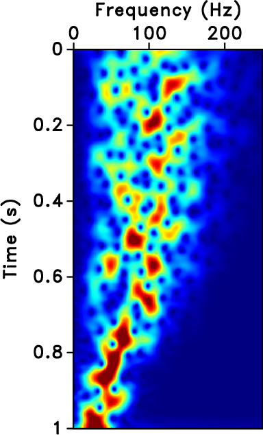
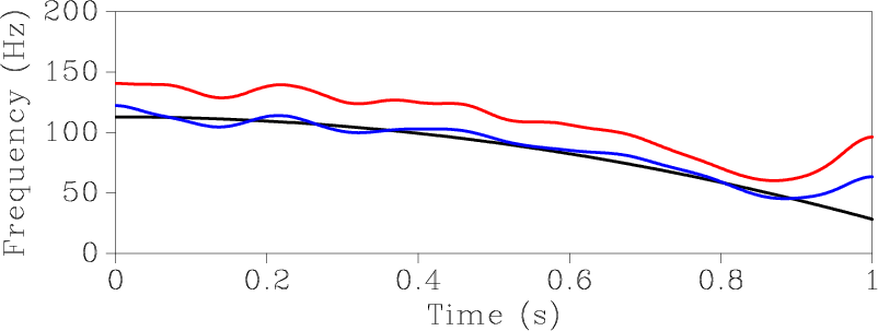
Figures 2b and 2c
show the time-frequency spectrum of the synthetic signal obtained
using the LTFT and S-transform, respectively. We estimated the local
centroid frequency from these two time-frequency spectra, as shown in
Figure 3 (the blue line is estimated from the LTFT, and the purple
line is estimated from the S-transform). Compared with the theoretical
centroid frequency (black line in Figures 2a
and 3), the local centroid frequency obtained using the
LTFT method is closer to the theoretical curve, so the LTFT analysis
method is selected for calculating the local centroid frequency and
time-varying Q-factors.
(Hu et al., 2013).
Figures 2b and 2c
show the time-frequency spectrum of the synthetic signal obtained
using the LTFT and S-transform, respectively. We estimated the local
centroid frequency from these two time-frequency spectra, as shown in
Figure 3 (the blue line is estimated from the LTFT, and the purple
line is estimated from the S-transform). Compared with the theoretical
centroid frequency (black line in Figures 2a
and 3), the local centroid frequency obtained using the
LTFT method is closer to the theoretical curve, so the LTFT analysis
method is selected for calculating the local centroid frequency and
time-varying Q-factors.
|
|---|
|
ref,sig
Figure 1. Theoretical model. Random reflectivity series (a), synthetic nonstationary signal (b). |
|
|
|
|---|
|
fpp,sigltft,sigst
Figure 2. Time-frequency spectrum. Theoretical time-frequency spectrum (the black line represents the theoretical centroid frequency) (a), time-frequency spectrum of the LTFT (b), time-frequency spectrum of the S-transform (c). |
|
|
|
|---|
|
difcf
Figure 3. Local centroid frequency estimation (the black line represents the theoretical centroid frequency, the blue line is estimated using the LTFT method, and the purple line is estimated using the S-transform). |
|
|
|
|
|
|
Continuous time-varying Q-factor estimation method in the time-frequency domain |