Continuous time-varying Q-factor estimation method in the time-frequency domain

Attenuated model with variable Q-factors

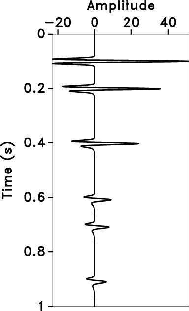
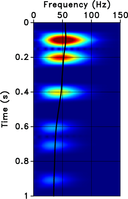
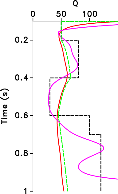
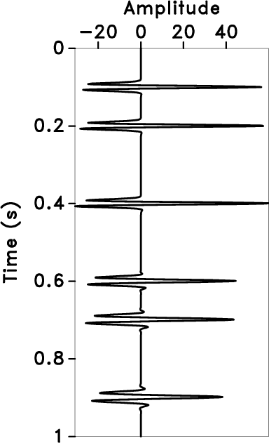
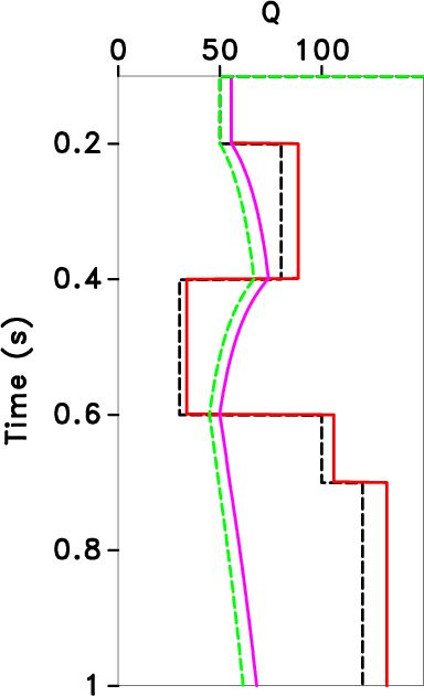
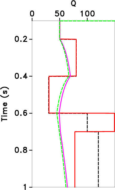
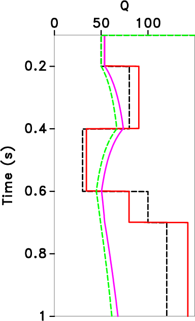
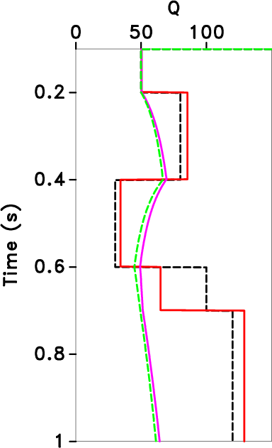
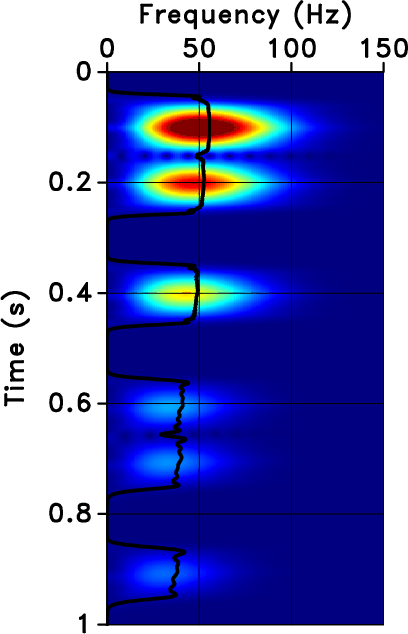
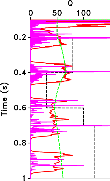
We synthesized an attenuated model with variable Q-factors to further verify the applicability of the proposed method. The time sampling interval of the synthetic signal is 1 ms, and there is a reflection interface at 0.1, 0.2, 0.4, 0.6, 0.7, and 0.9 s respectively. The attenuated seismic trace is synthesized according to the variable Q model (from 0 to 0.1 s, Q is infinite; from 0.1 to 0.2 s, Q is 50; from 0.2 to 0.4 s, Q is 80; from 0.4 to 0.6 s, Q is 30; from 0.6 to 0.7 s, Q is 100; from 0.7 to 0.9 s, Q is 120), as shown in Figure 9a. The timefrequency spectrum (Figure 9b) and the local centroid frequency (black line in Figure 9b) are obtained using the LTFT method. The results of the time-varying Q values (as shown in Figure 9c, the green dotted line represents the theoretical equivalent Q, the red line represents the estimated time-varying equivalent Q, the black dotted line represents the theoretical interval Q, and the purple line represents the time-varying interval Q calculated using the adjacent time information) using the LCFS method show that the error of the time-varying equivalent Q-factors estimated using this method is small and close to the trend of the theoretical equivalent Q-factors. However, the error of the time-varying interval Q-factors is large except for the third layer, which is mainly caused by the instability of the traditional Q-factor inversion method. Figure 9d shows the inverse Q filtering result calculated according to the time-varying equivalent Q, and the amplitude and phase of the wavelet are well compensated.

As with the attenuated model with constant Q, the proposed method is compared with the SR and CFS methods. We extract the spectrum information at the moment of the maximum amplitude in Figure 9b and estimate the interval Q-factors using the SR and CFS methods, as shown by the purple line in Figures 10a and 10b. Then, we change the picking time of the spectrum information. The Q-factors estimated using the SR and CFS methods are shown as purple lines in Figures 10c and  10d, respectively. It can be seen that the accuracy of the interface picking has a great influence on the estimated result of Q. The equivalent Q-factors are calculated according to the estimated interval Q-factors (the red lines in Figures 10a,  10b,  10c, and  10d). Compared with the time-varying equivalent Q-factors estimated using the LCFS method, the error of the traditional method is larger. The CFS method can also calculate continuous Q-factors without the extraction of interfaces. Figure 10e is the time-frequency spectrum of the attenuated signal ( Figure 9a), and the black line represents the instantaneous centroid frequency calculated using equation 3. We select the instantaneous centroid frequency at 0.1 s as the reference value and calculate the time-varying equivalent Q-factors (red line in Figure 10f) and the time-varying interval Q-factors (purple line in Figure 10f) based on the instantaneous centroid frequency. Compared with the LCFS method, this method can only obtain relatively accurate equivalent Q-factors when the spectrum is available. Moreover, the estimated time-varying interval Q-factors are extremely unstable.

vasignal,vfp,vqq,vcmsig
Figure 9. Attenuated modeland estimated results. The attenuated model with variable Q (a), the time-frequency spectrum of the LTFT (the black line represents the local centroid frequency) (b), Q estimated using the LCFS method (the green dotted line represents the theoretical equivalent Q, the red line represents the estimated time-varying equivalent Q, black dotted line represents the theoretical interval Q, and the purple line represents the estimated time-varying interval Q calculated) (c), inverse Q filtering result (d).

difsrq-1,difcfsq-1,difsrq-2,difcfsq-2,fp1,qq1
Figure 10. Q-factors estimated using different methods. The SR method (maximum amplitude) (a), CFS method (maximum amplitude) (b), SR method (nonmaximum amplitude) (c), CFS method (nonmaximum amplitude) (d), time-frequency spectrum of the LTFT (the black line represents the instantaneous centroid frequency) (e), Q estimated using the CFS method based on instantaneous centroid frequency (f).

Continuous time-varying Q-factor estimation method in the time-frequency domain