Continuous time-varying Q-factor estimation method in the time-frequency domain

Local centroid frequency shift (LCFS) method

Seismic waves propagating in underground media experience amplitude attenuation and phase distortion. High-frequency components attenuate faster than low-frequency components, so the centroid frequency of the amplitude spectrum experiences a downshift in the propagation process. Quan and Harris (1997) proposed the CFS method according to the above phenomenon.

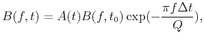
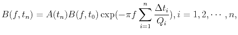
When considering seismic wave propagation in the viscoelastic medium, the amplitude spectrum of seismic waves with different travel times can be approximately expressed as (Zhang and Ulrych, 2002)

$$B(f,t)=A(t)B(f,t_0)\exp(-\frac{\pi f \Delta t}{Q}),$$ (12)

where Q is the quality factor, $\Delta t=t-t_0$ is the travel time difference , $A(t)$ is a frequency-independent factor (including spherical diffusion, transmission loss, etc.), $B(f,t_0)$ is the seismic amplitude spectrum at time $t_0$ , and $B(f,t)$ is the amplitude spectrum at travel time $t$ .

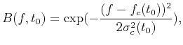
The CFS method assumes that the amplitude spectrum of the source wavelet satisfies the Gaussian distribution and can be expressed as

$$B(f,t_0)=\exp(-\frac{(f-f_c(t_0))^2}{2\sigma_c^2(t_0)}),$$ (13)

where $f_c(t_0)$ and $\sigma_c^2(t_0)$ represent the instantaneous centroid frequency and instantaneous variance of the amplitude spectrum at time $t_0$ , respectively. The timevarying Q-factors estimated using the CFS method can be obtained from equations 3, 4, and 12:

$$Q(t)=\frac{\pi\sigma_c^2(t_0)(t-t_0)}{f_c(t_0)-f_c(t)}.$$ (14)

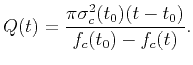
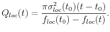
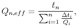
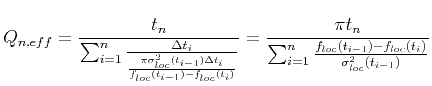
By replacing the instantaneous centroid frequency and instantaneous variance in equation 14 with the local centroid frequency and local variance, the time-varying Q-estimation equation can be rewritten as

$$Q_{loc}(t)=\frac{\pi\sigma_{loc}^2(t_0)(t-t_0)}{f_{loc}(t_0)-f_{loc}(t)}.$$ (15)

where $f_{loc}(t_0)$ and $\sigma_{loc}^2(t_0)$ represent the local centroid frequency and local variance of the amplitude spectrum at time $t_0$ , respectively, and $f_{loc}(t)$ is the local centroid frequency of the amplitude spectrum at time $t$ . The above method of estimating the Q values using the local centroid frequency is called the LCFS. It can be seen from the equation that this method must estimate the Q value in the time-frequency domain.

The CFS method assumes that the amplitude spectrum of the source wavelet is Gaussian spectrum and that the variance of the amplitude spectrum does not change with the attenuation effect. However, the amplitude spectrum of the actual seismic wave usually does not satisfy the Gaussian distribution. The absorption and attenuation effect would make the variance smaller and the bandwidth narrower, so the CFS method would produce the systematic error proportional to the travel time difference $\Delta t$ . When the travel time difference of the two reflected waves is small, the variances of the two waves are approximately equal. Thus, this paper improves the Q-estimation accuracy by reducing the travel time difference. Assuming that each time sampling point corresponds to a stratum interface, the above equation can be used to calculate the interval Q-factors between every two adjacent time sampling points. Then, the interval Q-factors can be used to further estimate the equivalent Q-factors between the reference and the target layers. The amplitude spectrum of layer $n$ can be expressed as (Zhang and Ulrych, 2002)

$$B(f,t_n)=A(t_n)B(f,t_0)\exp(-\pi f\sum_{i=1}^n\frac{\Delta t_i}{Q_i}), i=1,2,\cdots,n ,$$ (16)

where $\Delta t_i=t_i-t_{i-1}$ and $Q_i$ are the travel time and quality factor in layer $i$ , respectively.

The above equation can be expressed by the equivalent Q theory as

$$\exp(-\pi f\frac{t_n}{Q_{n,eff}})=\exp(-\pi f\sum_{i=1}^n\frac{\Delta t_i} {Q_i}),$$ (17)

The above equation can be simplifi ed to

$$Q_{n,eff}=\frac{t_n}{\sum_{i=1}^n\frac{\Delta t_i}{Q_i}},$$ (18)

where $t_n=\sum_{i=1}^n\Delta t_i$ represents the total travel time of a reflection.

By substituting the equation of interval Q-factors estimated using the LCFS method into the above equation, the equivalent Q-factor of layer $n$ ($n$ th time sampling point) can be expressed as

$$Q_{n,eff}=\frac{t_n}{\sum_{i=1}^n\frac{\Delta t_i}{\frac{\pi\sigm... ..._n} {\sum_{i=1}^n\frac{f_{loc}(t_{i-1})-f_{loc}(t_i)}{\sigma_{loc}^2(t_{i-1})}}$$ (19)

where $Q_{n,eff}$ represents the equivalent Q-factor from the reference layer to layer $n$ estimated using the LCFS method.

Continuous time-varying Q-factor estimation method in the time-frequency domain