|
|
|
|
High-order kernels for Riemannian Wavefield Extrapolation |
The first example is based on the Marmousi model
(Versteeg, 1994). We construct the coordinate system by ray
tracing from a point source at the surface in a smooth version of the
real velocity model. Figure 1 shows the velocity model with the
coordinate system overlaid, and Figures 2(a)-2(b) show
the coordinate system coefficients ![]() and
and ![]() defined in equations 11
and 12.
M-coswidth=0.80
Velocity map and Riemannian coordinate system for the Marmousi example.
defined in equations 11
and 12.
M-coswidth=0.80
Velocity map and Riemannian coordinate system for the Marmousi example.
|
|---|
|
M-abmRCa,M-abmRCb
Figure 1. Coordinate system coefficients defined in equations 11 and 12. (a) Parameter |
|
|
The goal of this test model is to illustrate the higher-order
extrapolation kernels in a fairly complex model using a simple
coordinate system. In this way, the coordinate system and the real
direction of wave propagation depart from one-another, thus accurate
extrapolation requires higher order kernels. The coordinate system is
constructed from a point at the location of the wave source. This
setting is similar to the case of extrapolation from a point source in
Cartesian coordinates, where high-angle
![]() propagation requires
high-order kernels.
propagation requires
high-order kernels.
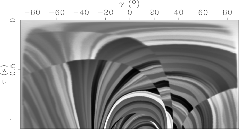
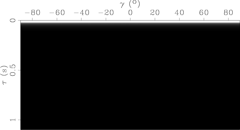
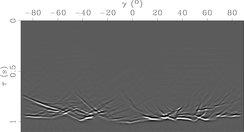
Figures 3(a)-3(d) show impulse responses for a
point source computed with various extrapolators in ray coordinates
(![]() and
and ![]() ). Panels (a) and (c) show extrapolation with the
). Panels (a) and (c) show extrapolation with the
![]() and
and ![]() , respectively. Panels (b) and (d) show
extrapolation with the pseudo-screen (PSC) equation, and the Fourier
finite-differences (FFD) equation, respectively. All plots are
displayed in ray coordinates. We can observe that the angular accuracy
of the extrapolator improves for the more accurate extrapolators. The
finite-differences solutions (panels a and c) show the typical
behavior of such solutions for the
, respectively. Panels (b) and (d) show
extrapolation with the pseudo-screen (PSC) equation, and the Fourier
finite-differences (FFD) equation, respectively. All plots are
displayed in ray coordinates. We can observe that the angular accuracy
of the extrapolator improves for the more accurate extrapolators. The
finite-differences solutions (panels a and c) show the typical
behavior of such solutions for the ![]() and
and ![]() equations
(e.g. the cardioid for
equations
(e.g. the cardioid for ![]() ), but in the more general setting
of Riemannian extrapolation. The mixed-domain extrapolators (panels b
and d) are more accurate the finite-differences extrapolators. The
main differences occur at the highest propagation angles. As for the
case of Cartesian extrapolation, the most accurate kernel of those
compared is the equivalent of Fourier finite-differences.
), but in the more general setting
of Riemannian extrapolation. The mixed-domain extrapolators (panels b
and d) are more accurate the finite-differences extrapolators. The
main differences occur at the highest propagation angles. As for the
case of Cartesian extrapolation, the most accurate kernel of those
compared is the equivalent of Fourier finite-differences.
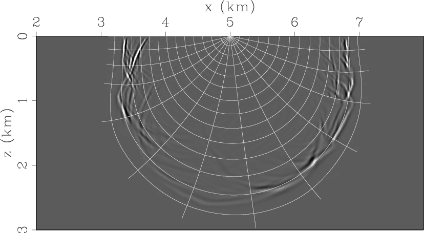
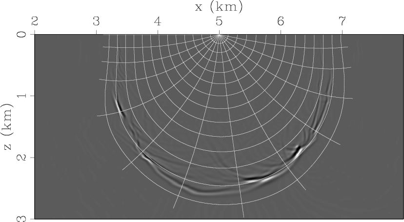
Figures 4(a)-4(d) show the corresponding plots in Figures 3(a)-3(d) mapped in the physical coordinates. The overlay is an outline of the extrapolation coordinate system. After re-mapping to the physical space, the comparison of high-angle accuracy for the various extrapolators is more apparent, since it now has physical meaning.
Figures 5(a)-5(b) show a side-by-side comparison of
equivalent extrapolators in Riemannian and Cartesian coordinates. The
impulse response in Figure 5(a) shows the limits of Cartesian
extrapolation in propagating waves correctly up to ![]() . The
Riemannian extrapolator in Figure 5(b) handles much better waves
propagating at high angles, including energy that is propagating
upward relative to the physical coordinates.
. The
Riemannian extrapolator in Figure 5(b) handles much better waves
propagating at high angles, including energy that is propagating
upward relative to the physical coordinates.


|
|---|
|
M-migRC-F15,M-migRC-PSC,M-migRC-F60,M-migRC-FFD
Figure 2. Migration impulse responses in Riemannian coordinates. (a) Extrapolation with the |
|
|


|
|---|
|
M-migCC-F15,M-migCC-SSF,M-migCC-F60,M-migCC-FFD
Figure 3. Migration impulse responses in Riemannian coordinates after mapping to Cartesian coordinates. (a) Extrapolation with the |
|
|
|
|---|
|
M-imgCC,M-migCC-SSF
Figure 4. Comparison of extrapolation in Cartesian and Riemannian coordinates. (a) Split-step Fourier extrapolation in Cartesian coordinates. (b) Split-step Fourier extrapolation in Riemannian coordinates. |
|
|
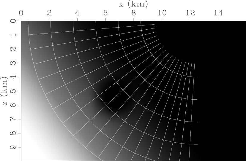
The second example is based on a model with a large lateral gradient
which makes an incident plane wave overturn. A small Gaussian anomaly,
not used in the construction of the coordinate system, forces the
propagating wave to triplicate and move at high angles relative to the
extrapolation direction. Figure 6 shows the velocity model with the
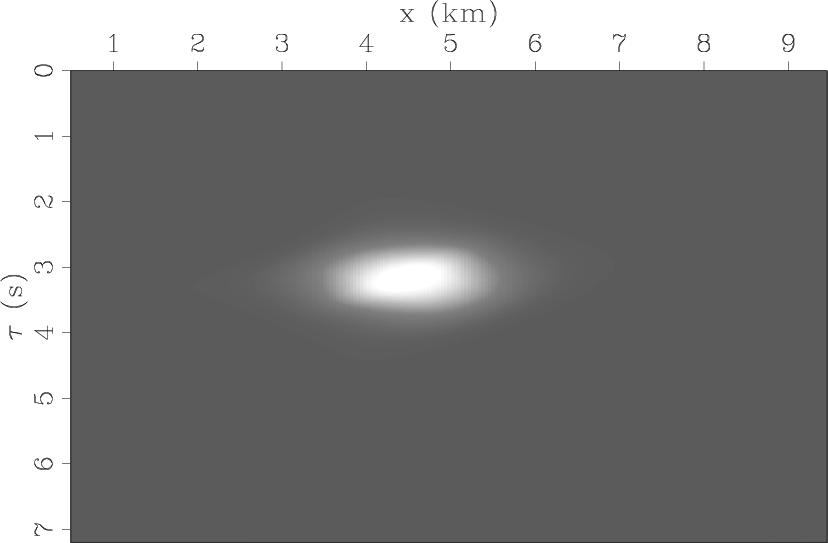
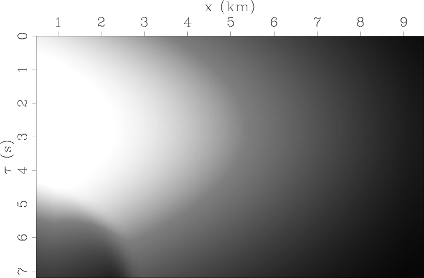
coordinate system overlaid. Figures 7(a)-7(b) show the
coordinate system coefficients, ![]() and
and ![]() defined in equations 11 and
12.
defined in equations 11 and
12.
|
|---|
|
D-cos
Figure 5. Velocity map and Riemannian coordinate system for the large-gradient model experiment. |
|
|
|
|---|
|
D-abmRCa,D-abmRCb
Figure 6. Coordinate system coefficients defined in equations 11 and 12. (a) Parameter |
|
|
The goal of this model is to illustrate Riemannian wavefield extrapolation in a situation which cannot be handled correctly by Cartesian extrapolation, no matter how accurate an extrapolator we use. In this example, an incident plane wave is overturning, thus becoming evanescent for the solution constructed in Cartesian coordinates. Furthermore, the Gaussian anomaly shown in Figure 7(a) causes wavefield triplication, thus requiring high-order kernels for the Riemannian extrapolator.
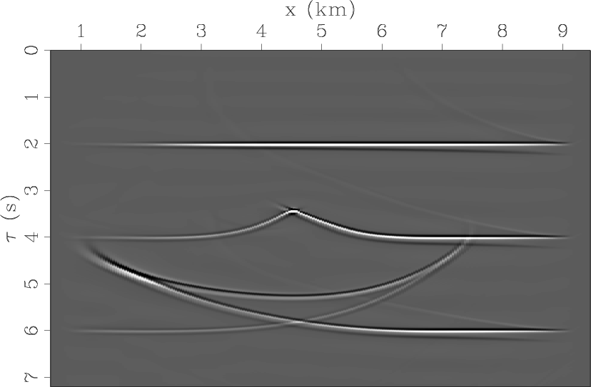
Figures 8(a)-8(d) show impulse responses for an
incident plane wave computed with various extrapolators in ray
coordinates (![]() and
and ![]() ). Panels (a) and (c) show extrapolation
with the
). Panels (a) and (c) show extrapolation
with the ![]() and
and ![]() finite-differences equations,
respectively. Panel (b) and (d) show extrapolation with the
pseudo-screen (PSC) equation and the Fourier finite-differences (FFD)
equation, respectively. All plots are displayed in ray coordinates. As
for the preceding example, we observe higher angular accuracy as we
increase the order of the extrapolator. The equivalent FFD
extrapolator shows the highest accuracy of all tested extrapolators.
finite-differences equations,
respectively. Panel (b) and (d) show extrapolation with the
pseudo-screen (PSC) equation and the Fourier finite-differences (FFD)
equation, respectively. All plots are displayed in ray coordinates. As
for the preceding example, we observe higher angular accuracy as we
increase the order of the extrapolator. The equivalent FFD
extrapolator shows the highest accuracy of all tested extrapolators.
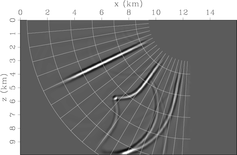
As in the preceding example, Figures 9(a)-9(d) show the corresponding plots in Figures 8(a)-8(d) mapped in the physical coordinates. The overlay is an outline of the extrapolation coordinate system.
Finally, Figures 10(a) and 10(b) show a side-by-side
comparison of equivalent extrapolators in Riemannian and Cartesian
coordinates. The impulse response in Figure 10(a) clearly shows
the failure of the Cartesian extrapolator in propagating waves
correctly even up to ![]() . The Riemannian extrapolator in
Figure 10(b) handles much better overturning waves, including
energy that is propagating upward relative to the vertical direction.
. The Riemannian extrapolator in
Figure 10(b) handles much better overturning waves, including
energy that is propagating upward relative to the vertical direction.


|
|---|
|
D-migRC-F15,D-migRC-PSC,D-migRC-F60,D-migRC-FFD
Figure 7. Migration impulse responses in Riemannian coordinates. (a) Extrapolation with the |
|
|


|
|---|
|
D-migCC-F15,D-migCC-PSC,D-migCC-F60,D-migCC-FFD
Figure 8. Migration impulse responses in Riemannian coordinates after mapping to Cartesian coordinates. (a) Extrapolation with the |
|
|


|
|---|
|
D-imgCC-bp,D-migCC-SSF
Figure 9. Comparison of extrapolation in Cartesian and Riemannian coordinates. (a) Split-step Fourier extrapolation in Cartesian coordinates. (b) Split-step Fourier extrapolation in Riemannian coordinates. |
|
|
|
|
|
|
High-order kernels for Riemannian Wavefield Extrapolation |