 |
 |
 |
 | High-order kernels for Riemannian Wavefield Extrapolation |  |
![[pdf]](icons/pdf.png) |
Next: Examples
Up: Extrapolation kernels
Previous: Space-domain extrapolation
Mixed-domain solutions to the one-way wave equation consist of
decompositions of the extrapolation wavenumber defined in
equation 13 in terms computed in the Fourier domain for a reference
of the extrapolation medium, followed by a finite-differences
correction applied in the space-domain. For equation 13, a generic
mixed-domain solution has the form:
 |
(13) |
where  and
and  are reference values for the medium
characterized by the parameters
are reference values for the medium
characterized by the parameters  and
and  , and the coefficients
 ,
,  and
and  take different forms according to the type of
approximation. As for usual Cartesian coordinates,
take different forms according to the type of
approximation. As for usual Cartesian coordinates,  is applied
in the Fourier domain, and the other two terms are applied in the
space domain. If we limit the space-domain correction to the thin lens
term,
is applied
in the Fourier domain, and the other two terms are applied in the
space domain. If we limit the space-domain correction to the thin lens
term,
 , we obtain the equivalent of the split-step
Fourier (SSF) method (Stoffa et al., 1990) in Riemannian
coordinates.
, we obtain the equivalent of the split-step
Fourier (SSF) method (Stoffa et al., 1990) in Riemannian
coordinates.
Appendix A details the derivations for two types of expansions known
by the names of pseudo-screen (Huang et al., 1999), and Fourier
finite-differences (Biondi, 2002; Ristow and Ruhl, 1994). Other
extrapolation approximations are possible, but are not described here,
for simplicity.
- Pseudo-screen method:
The coefficients for the pseudo-screen approximation to equation 21 are
&=& a_0[c_1(aa_0-1 )- (bb_0-1 )](b_0a_0)^2,
&=& 1 ,
&=&3c_2(b_0a_0)^2,
where and are reference values for the medium
characterized by parameters and . In the special case of
Cartesian coordinates,  and
and  , equation 21 with
coefficients equation 22 takes the familiar form
, equation 21 with
coefficients equation 22 takes the familiar form
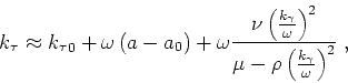
![\begin{displaymath}
k_\tau \approx {k_\tau }_0+ \omega
\left [1+ \frac{ \frac{...
...ma }{ \omega } \right )^2}
\right ] \left (s-s_0 \right )\;,
\end{displaymath}](img63.png) |
(14) |
where the coefficients  and
and  take different values for
different orders of the finite-differences term:
take different values for
different orders of the finite-differences term:
 ,
,
 , etc. When
 we obtain the usual split-step Fourier
equation (Stoffa et al., 1990).
we obtain the usual split-step Fourier
equation (Stoffa et al., 1990).
- Fourier finite-differences method:
The coefficients for the Fourier finite-differences solution to equation 21 are
&=& 12_1^2 ,
&=& _1 ,
&=& 14_2 ,
where, by definition,
_1 &=& a(b a )^2- a_0(b_0a_0)^2,
_2 &=& a(b a )^4- a_0(b_0a_0)^4.
and are reference values for the medium characterized by
the parameters and . In the special case of Cartesian
coordinates, and , equation 21 with coefficients
equation 26 takes the familiar form:
![\begin{displaymath}
k_\tau \approx {k_\tau }_0+ \omega
\left [1+ \frac{ \frac{...
...ma }{ \omega } \right )^2}
\right ] \left (s-s_0 \right )\;,
\end{displaymath}](img65.png) |
(15) |
where the coefficients and take different values for
different orders of the finite-differences term:
for  ,
for
,
for
 , etc. When
  we obtain the usual split-step
Fourier equation (Stoffa et al., 1990).
we obtain the usual split-step
Fourier equation (Stoffa et al., 1990).
|
|
|
|
| High-order kernels for Riemannian Wavefield Extrapolation | |
|
Next: Examples
Up: Extrapolation kernels
Previous: Space-domain extrapolation
2008-12-02