High-order kernels for Riemannian Wavefield Extrapolation

Riemannian wavefield extrapolation

Riemannian wavefield extrapolation (Sava and Fomel, 2005) generalizes solutions to the Helmholtz equation of the acoustic wave-equation

$$\DEL u=-\omega ^2 s^2 u\;,$$ (1)

to coordinate systems that are different from simple Cartesian, where extrapolation is performed strictly in the downward direction. In equation 1, $s$ is slowness, $\omega$ is temporal frequency, and $u$ is a monochromatic acoustic wave. The Laplacian operator $\Delta$ takes different forms according to the coordinate system used for discretization.

Assume that we describe the physical space in Cartesian coordinates $x$, $y$ and $z$, and that we describe a Riemannian coordinate system using coordinates $\xi$, $\eta$ and $\zeta$. The two coordinate systems are related through a mapping x&=&x(,,)
y&=&y(,,)
z&=&z(,,) which allows us to compute derivatives of the Cartesian coordinates relative to the Riemannian coordinates.

A special case of the mapping 2-4 is defined when the Riemannian coordinate system is constructed by ray tracing. The coordinate system is defined by traveltime $\tau$ and shooting angles, for example. Such coordinate systems have the property that they are semi-orthogonal, i.e. one axis is orthogonal on the other two, although the later axes are not necessarily orthogonal on one-another.

Following the derivation in Sava and Fomel (2005), the acoustic wave-equation in Riemannian coordinates can be written as:

$$c_{\zeta \zeta }\frac{\partial^2 u}{\partial \zeta ^2} + c_{... ...partial \xi \partial\eta } = - \left (\omega s \right)^2 u\;,$$ (2)

where coefficients $c_{ij}$ are functions of the coordinate system and can be computed numerically for any given coordinate system mapping 2-4.

The acoustic wave-equation in Riemannian coordinates 5 contains both first and second order terms, in contrast with the normal Cartesian acoustic wave-equation which contains only second order terms. We can construct an approximate Riemannian wavefield extrapolation method by dropping the first-order terms in equation 5. This approximation is justified by the fact that, according to the theory of characteristics for second-order hyperbolic equations (Courant and Hilbert, 1989), the first-order terms affect only the amplitude of the propagating waves. To preserve the kinematics, it is sufficient to retain only the second order terms of equation 5:

$$c_{\zeta \zeta }\frac{\partial^2 u}{\partial \zeta ^2} + c_{... ...partial \xi \partial\eta } = - \left (\omega s \right)^2 u\;.$$ (3)

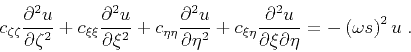
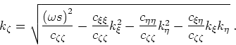
From equation 6 we can derive the following dispersion relation of the acoustic wave-equation in Riemannian coordinates

$$- c_{\zeta \zeta }k_\zeta ^2 - c_{\xi \xi }k_\xi ^2 - c_{\et... ... c_{\xi \eta }k_\xi k_\eta = - \left (\omega s \right )^2 \;,$$ (4)

where $k_\zeta$, $k_\xi$ and $k_\eta$ are wavenumbers associated with the Riemannian coordinates $\zeta$, $\xi$ and $\eta$. Coefficients $c_{\xi \xi }$, $c_{\eta \eta }$ and $c_{\zeta \zeta }$ are known quantities defined using the coordinate system mapping 2-4. For one-way wavefield extrapolation, we need to solve the quadratic equation 7 for the wavenumber of the extrapolation direction $k_\zeta$, and select the solution with the appropriate sign for the desired extrapolation direction:

$$k_\zeta = \sqrt{ \frac{ \left (\omega s\right )^2}{c_{\zeta... ...^2 - \frac{c_{\xi \eta }}{c_{\zeta \zeta }}k_\xi k_\eta }\;.$$ (5)

The 2D equivalent of equation 8 takes the form:

$$k_\zeta = \sqrt{ \frac{ \left (\omega s\right )^2}{c_{\zeta \zeta }} - \frac{c_{\xi \xi }}{c_{\zeta \zeta }}k_\xi ^2 }\;.$$ (6)

In ray coordinates, defined by $\zeta \equiv \tau$ (propagation time) and $\xi \equiv \gamma$ (shooting angle), we can re-write equation 9 as

$$k_\tau = \sqrt{ \left (\omega s {\bf a}\right)^2 - \left (\frac{{\bf a}}{{\bf j}} {\bf k}\right)^2 }\;,$$ (7)

where ${\bf a}$ represents velocity and ${\bf j}$ represents geometrical spreading. The quantities ${\bf a}$ and ${\bf j}$ characterize the extrapolation coordinate system: ${\bf a}$ describes the velocity used for construction of ray coordinate system; ${\bf j}$ describes the spreading or focusing of the coordinate system. In general, the velocity used for construction of the coordinate system is different from the velocity used for extrapolation, as suggested by Sava and Fomel (2005) and illustrated later in this paper.

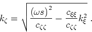
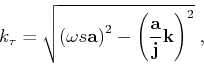
We can further simplify the computations by introducing the notation a &=& s a,
b &=& aj , thus equation 10 taking the form

$$k_\tau = \sqrt{ \left (\omega a \right)^2 - \left (b{\bf k}\right)^2} \;.$$ (8)

For Cartesian coordinate systems, ${\bf a}=1$ and ${\bf j}=1$, equation 13 reduces to the known dispersion relation

$$k_z = \sqrt{\omega ^2 s^2 - k_x^2} \;,$$ (9)

where $k_z$ and $k_x$ are depth and position extrapolation wavenumbers.

High-order kernels for Riemannian Wavefield Extrapolation