|
|
|
|
A variational approach for picking optimal surfaces from semblance-like panels |
|
|---|
|
viking-cmps,viking-envelope-f
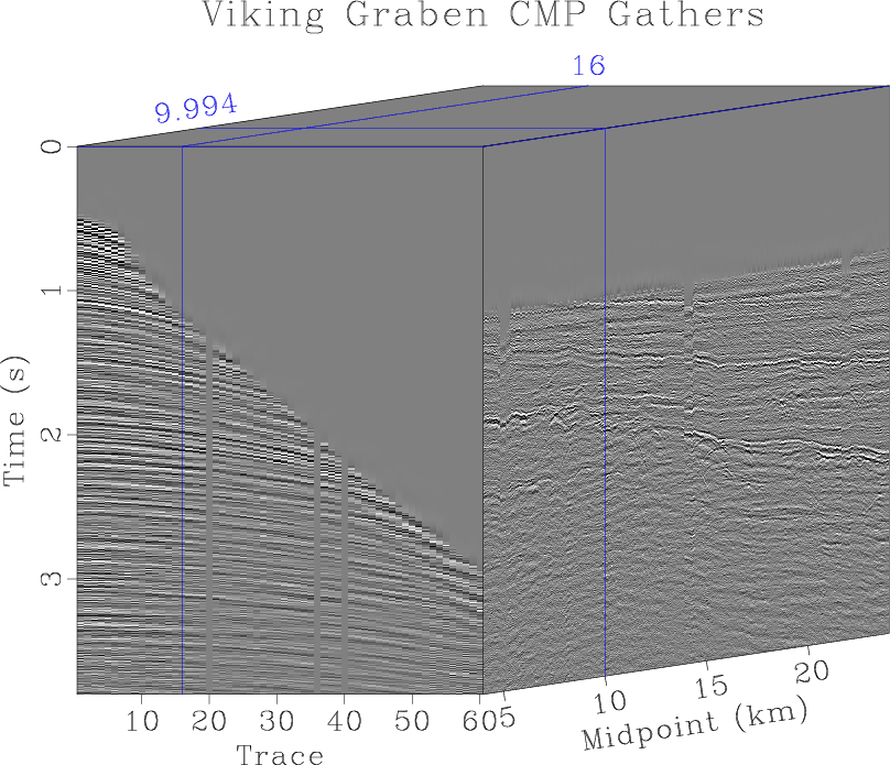
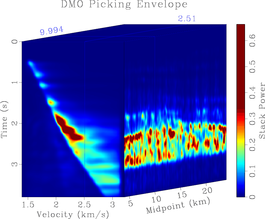
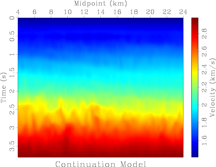
Figure 1. (a) Common midpoint gathers from the Viking Graben; (b) Constant velocity DMO stack power. |
|
|
We apply the method to a field data example from the Viking Graben featured in Keys and Foster (1998). Figure 1a contains a set of common midpoint (CMP) gathers which were preprocessed to have multiples removed for times less than 2 seconds (s) using the parabolic Radon transform.
We apply the DMO method from Fowler (1988) to generate a series of constant-velocity stacks from which the stack power, or envelope, is computed. This will serve as
![]() . A lower mute is applied to suppress high envelope values corresponding to multiples below 2 s. Triangle smoothing and scaling, featuring smoothing radii ranging in strength from
. A lower mute is applied to suppress high envelope values corresponding to multiples below 2 s. Triangle smoothing and scaling, featuring smoothing radii ranging in strength from
![]() to
to
![]() and scaling factors ranging from
and scaling factors ranging from ![]() to
to ![]() , are applied to the muted volume for use in continuation. The least-smoothed version is shown in Figure 1b. We generate 10 volumes of increasingly aggressive smoothing and scaling and apply the
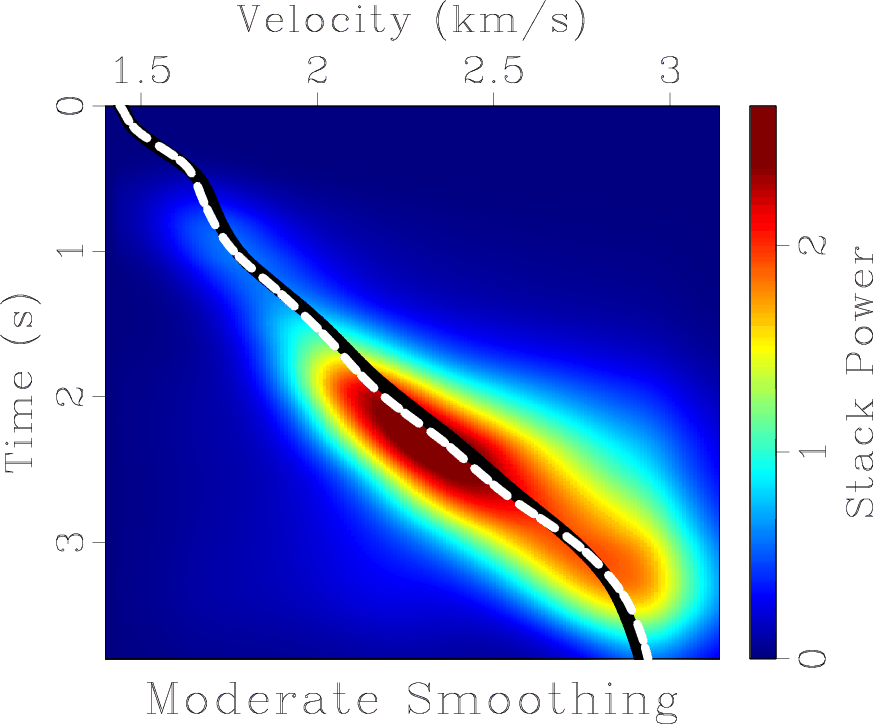
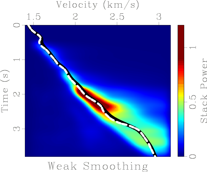
, are applied to the muted volume for use in continuation. The least-smoothed version is shown in Figure 1b. We generate 10 volumes of increasingly aggressive smoothing and scaling and apply the ![]() -BFGS variational velocity picking algorithm with continuation using those volumes. The picking algorithm is allowed to proceed for a maximum of 20 iterations at each continuation level. The initial continuation level is shown in Figure 2a. The initial model shown in solid black is a linear
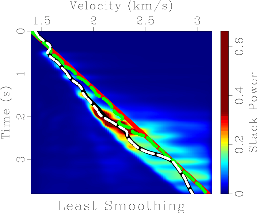
-BFGS variational velocity picking algorithm with continuation using those volumes. The picking algorithm is allowed to proceed for a maximum of 20 iterations at each continuation level. The initial continuation level is shown in Figure 2a. The initial model shown in solid black is a linear ![]() spanning the range of scanned velocities and record times. The final model of this continuation level is shown in dashed white. The sixth continuation level is shown in Figure 2b, the ninth in Figure 2c, and the tenth and final level in Figure 2d. In each of these panels, the solid black line represents the starting model for the continuation level, which was the final model of the previous one, and the dashed white line is the final model. Figure 2d also features the linear initial model in solid red, which is the same as the starting model in Figure 2a, and the picking output without continuation in dashed green. This model is generated applying the
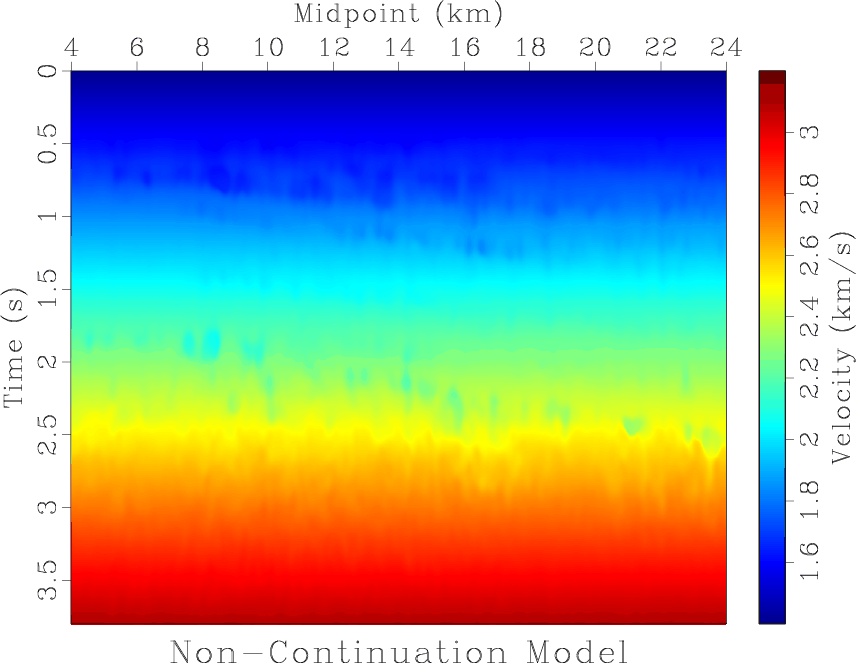
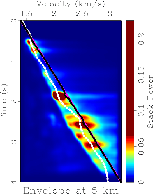
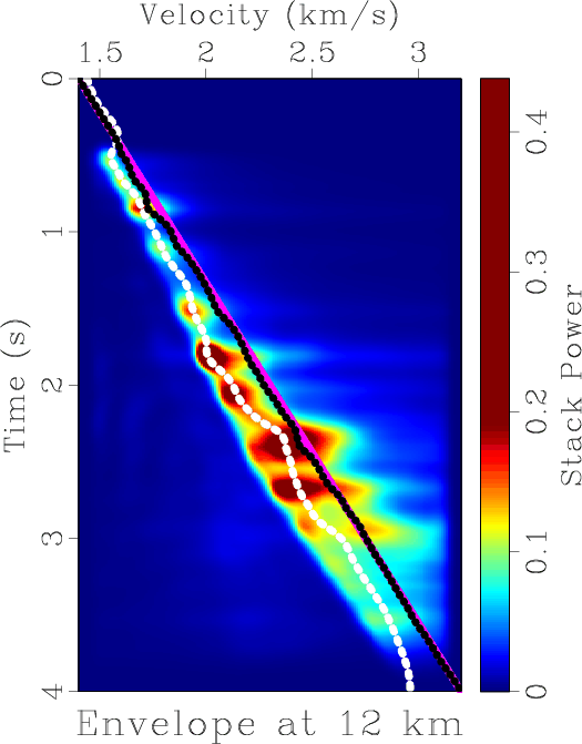
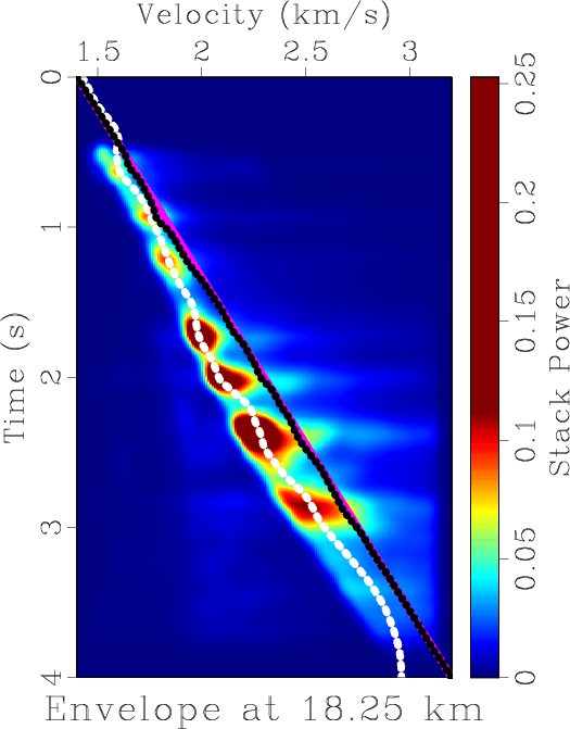
spanning the range of scanned velocities and record times. The final model of this continuation level is shown in dashed white. The sixth continuation level is shown in Figure 2b, the ninth in Figure 2c, and the tenth and final level in Figure 2d. In each of these panels, the solid black line represents the starting model for the continuation level, which was the final model of the previous one, and the dashed white line is the final model. Figure 2d also features the linear initial model in solid red, which is the same as the starting model in Figure 2a, and the picking output without continuation in dashed green. This model is generated applying the ![]() -BFGS picking approach only on this level of smoothing, again with a maximum of 20 iterations. This non-continuation final model is shown in Figure 3a, and the final model with continuation is displayed in Figure 3b. To further illustrate how the two final models track stack power at different positions within the study area, overlays of the starting model (solid fuchsia), non-continuation final model (dashed black) and continuation final model (dashed white) are plotted on stack power at midpoints of 5 km in Figure 4a, 12 km in Figure 4b and 18.25 km in Figure 4c. The cost functional in Equation 4 is evaluated for each update of both methods using the least-smoothed stack power volume visible in Figure 1b.
-BFGS picking approach only on this level of smoothing, again with a maximum of 20 iterations. This non-continuation final model is shown in Figure 3a, and the final model with continuation is displayed in Figure 3b. To further illustrate how the two final models track stack power at different positions within the study area, overlays of the starting model (solid fuchsia), non-continuation final model (dashed black) and continuation final model (dashed white) are plotted on stack power at midpoints of 5 km in Figure 4a, 12 km in Figure 4b and 18.25 km in Figure 4c. The cost functional in Equation 4 is evaluated for each update of both methods using the least-smoothed stack power volume visible in Figure 1b.
Notice that the cost for each model never attains zero. This is because the cost defined by Equation 4 is related to the regularized, incremental surface area of the velocity model,
 weighted by
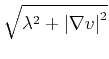
![]() at each model position with an additional total variation term
at each model position with an additional total variation term
![]() . Here,
. Here,
![]() is the stack power volume at zero-offset time
is the stack power volume at zero-offset time ![]() , midpoint
, midpoint ![]() , and model velocity
, and model velocity ![]() . Since stack power is positive and bounded above by some
. Since stack power is positive and bounded above by some
![]() ,
,
![]() . The surface area term is always greater than or equal to
. The surface area term is always greater than or equal to ![]() , and the total variation term is greater than or equal to zero. Thus, the lowest cost a model could possibly attain is
, and the total variation term is greater than or equal to zero. Thus, the lowest cost a model could possibly attain is
![]() where
where ![]() is the difference between maximum and minimum zero-offset time for the stack power volume and
is the difference between maximum and minimum zero-offset time for the stack power volume and ![]() is the difference between the maximum and minimum midpoint. For this example, that bounding minimal cost is roughly 40, but that would entail a constant velocity model through a stack power volume uniformly containing maximum stack power values which, on examination of Figure 1b, is clearly not the case. In effect, the cost function, and consequently the update at each iteration, seeks the model that balances tracking high stack power values with minimal model variation.
is the difference between the maximum and minimum midpoint. For this example, that bounding minimal cost is roughly 40, but that would entail a constant velocity model through a stack power volume uniformly containing maximum stack power values which, on examination of Figure 1b, is clearly not the case. In effect, the cost function, and consequently the update at each iteration, seeks the model that balances tracking high stack power values with minimal model variation.
|
|---|
|
viking-velo-gather-0,viking-velo-gather-5,viking-velo-gather-8,viking-velo-gather-9
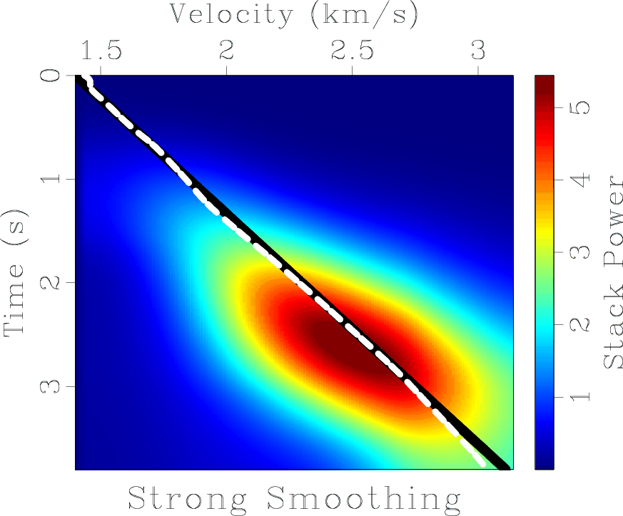
Figure 2. Illustration of continuation picking for midpoint at 9.994 km. Solid black line plots starting model for each level, dashed white line shows final model. (a) Initial continuation level with strongest smoothing; (b) Middle continuation level with moderate smoothing; (c) Second to last continuation level with weak smoothing; (d) Final continuation level also plotting the initial (solid red) and final models (dashed green) for picking without continuation. |
|
|
|
|---|
|
viking-no-continuation-velo,viking-velo-out-9
Figure 3. (a) Velocity model determined by variational picking algorithm without continuation; (b) Velocity model determined by variational velocity picking algorithm utilizing continuation. |
|
|
|
|---|
|
gather-0,gather-5,gather-8
Figure 4. Illustration of the picking output at: (a) 5 km; (b) 12 km; (c) 18.25 km. Solid fuchsia line plots the starting model, dashed black line plots the non-continuation final model from Figure 3a, dashed white line plots the continuation final model from Figure 3b. Background plots the stack power with minimal smoothing shown in Figure 1b. |
|
|
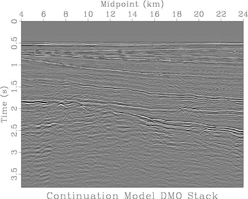
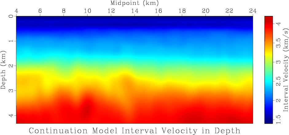
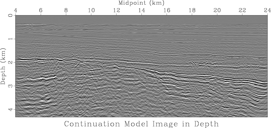
We use the continuation velocity field to DMO stack the data, as shown in Figure 5a. Then we apply Kirchhoff migration to the data, as displayed in Figure 5b. The Dix formula (Dix, 1955) is used to compute interval velocity for the continuation model. This is a representation of local velocity through material at each region in the subsurface. Picked velocities are RMS velocities, corresponding to a mean velocity value over the complete ray path. The interval velocity is used for conversion from the time to the depth domain following the manner of Sripanich and Fomel (2018). The depth stretched interval velocity for the continuation model is plotted in Figure 6a and the corresponding depth stretched image in Figure 6b.

|
|---|
|
viking-velo-out-9-slice,viking-velo-out-9-slice-img
Figure 5. (a) DMO stack of the data set in Figure 1a using the continuation velocity model from Figure 3b; (b) Kirchhoff time migrated images of the DMO stack in Figure 5a using the continuation velocity model in Figure 3b. |
|
|
Notice that continuation behaves as a more global optimization scheme, enabling the solution to avoid local minima. In fact, on the first continuation level shown in Figure 2a, the cost actually increases when calculated on the least-smoothed stack power volume, as shown in Figure ![]() . This enables the continuation velocity model to find the dominant trend where it deviates from the starting model, and produce a final model with a low associated cost. The model found without continuation is only able to follow stack power highs where the starting model is already near those highs, as can be seen around 2.25 s in Figure 2d, and in the three positions illustrated in Figures 4a, 4b, and 4c, where the black non-continuation final model primarily either overlies or is close to the initial model shown in fuchsia. The velocity field computed without continuation finds a local minimum with higher cost than the one found using continuation, as shown in Figure
. This enables the continuation velocity model to find the dominant trend where it deviates from the starting model, and produce a final model with a low associated cost. The model found without continuation is only able to follow stack power highs where the starting model is already near those highs, as can be seen around 2.25 s in Figure 2d, and in the three positions illustrated in Figures 4a, 4b, and 4c, where the black non-continuation final model primarily either overlies or is close to the initial model shown in fuchsia. The velocity field computed without continuation finds a local minimum with higher cost than the one found using continuation, as shown in Figure ![]() .
.
|
|---|
|
viking-velo-out-9-dix-depthmapped-aspect-bar,viking-velo-out-9-slice-img-depthmapped-aspect
Figure 6. (a) Interval velocity corresponding to continuation model in Figure 3b transformed to the depth domain; (b) Continuation model image in Figure 5b transformed to the depth domain. |
|
|
The velocity field determined using continuation, Figure 3b, appears geologically plausible. Velocity values vary smoothly even though smoothness was not explicitly imposed. Furthermore, the velocity values in that model are in agreement with velocities computed from vertical seismic profile (VSP) travel time curves for two wells along the seismic line featured in Keys and Foster (1998). Seismic events in the DMO stack, Figure 5a, and seismic image, Figure 5b, generated using that model tend to be well-focused. Additionally, depth domain interval velocity traces for the continuation model displayed in Figure 6a match the trend of sonic log p-wave velocities at the two well locations along the line (Keys and Foster, 1998).
|
|
|
|
A variational approach for picking optimal surfaces from semblance-like panels |