|
|
|
|
Probabilistic moveout analysis by time warping |
Next: Examples Up: Theory Previous: 3D generalized nonhyperboloidal moveout
|
|
|
|
Probabilistic moveout analysis by time warping |
Equipped with the general concepts on time-warping and the choice of 3D GMA described in the previous sections, we propose to solve this moveout inversion problem with a global Monte Carlo inversion method. This choice is encouraged by the non-uniqueness of the solution of this inverse problem that only relies on traveltime (kinematic) data and the fact that the 3D GMA depends non-linearly on associated moveout parameters. By employing a global optimization scheme within a Bayesian framework, we can map out the non-uniqueness of possible solutions and present them as posterior probability distributions, while also honoring the non-linearity of the problem. Here, we largely follow the notations of Mosegaard and Tarantola (1995) and Tarantola (2005), where we express the posterior probability density function
 as
as
 denotes the prior probability density function of model parameters
 and
and
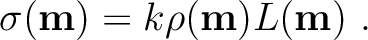
 represents the likelihood function (with an appropriate normalization constant
  ) that measures the degree of fit between predicted data and observed data. Assuming a prior
that we can draw samples from, the goal is to design a selection process based on
that will result in samples whose density directly represents
.
) that measures the degree of fit between predicted data and observed data. Assuming a prior
that we can draw samples from, the goal is to design a selection process based on
that will result in samples whose density directly represents
.
Mosegaard and Tarantola (1995) showed that given samples of
and a choice of
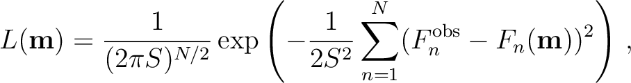
, the selection process can be done by means of the Metropolis-Hastings algorithm. In this study, we define
as:
 , the misfit between the observed
 and modeled
 for all
  traces in the considered CMP gather is evaluated and summed according to equation 7. Here,
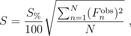
  represents a `hyperparameter' related to data uncertainty, which we choose to express as
with
represents a `hyperparameter' related to data uncertainty, which we choose to express as
with  denoting the magnitude of uncertainty expressed in percent with respect to the root mean square (RMS) of the data
. Because is constant for each CMP event, can also be considered as a relative uncertainty in the estimated reflection traveltime squared (equation 2).
denoting the magnitude of uncertainty expressed in percent with respect to the root mean square (RMS) of the data
. Because is constant for each CMP event, can also be considered as a relative uncertainty in the estimated reflection traveltime squared (equation 2).
We emphasize that data uncertainty is generally not easily quantified in practice due to the workflow of estimating  . To account for this complication, we propose to utilize the transdimensional (hierarchical Bayesian) inversion framework (Sambridge et al., 2006; Malinverno and Briggs, 2004; Sambridge et al., 2013), which permits us to treat as yet another parameter to be estimated during the inversion. In this way, we obviate the need to estimate the data uncertainty explicitly, while correctly honoring its effects in our inversion. Our implementation of the Monte Carlo inversion with Metropolis-Hastings rule can, therefore, be summarized as follows:
 with a guess set of
 drawn from the prior distributions of each model parameter. In the case of the 3D GMA,
consists of
drawn from the prior distributions of each model parameter. In the case of the 3D GMA,
consists of  ,
,  ,
,  ,
,  , and . For uniform prior distributions, a random number generator can be used for drawing samples; whereas, for Gaussian prior distributions, a combination of a random number generator and the Box-Muller transform can be used.
 according to equation 7 with a choice of cutoff offset that depends on the example at hand.
 with a new guess of
 drawn from the same distribution. This attempt is evaluated according to the following Metropolis-Hastings rule.
 , then accept the move to .
 , then make a random decision of staying at or accepting the move to with a probability of
  .
.
after the selection.
In our workflow, we propose to perform moveout parameter estimation with two inversion runs:
using only small-offset data. At this stage, we assume that the prior distribution is uniform within the chosen bounds (min and max values) for each model parameter in
and specify a small cutoff offset (e.g., where the offset-to-depth ratio is assumed to be unity).
from the first run are assumed to be Gaussian and will be used as new prior distributions for in the second inversion run with all available (small- and large-offsets) data to estimate , , and . Better prior distributions of from the first run are expected to help with the estimation of , , and . The prior distributions for other pertaining parameters are again assumed to be uniform within some chosen bounds (min and max values).
After the two runs, the final recorded
can be visualized as histograms that represent 1D marginal posterior probability distributions of the estimated moveout parameters
. The corresponding posterior probability density function
can subsequently be obtained with appropriate normalization of the histograms. In order to quantify the `gain of information' from the moveout inversion process, we use the Kullback-Leibler divergence
 given by,
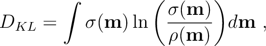 |
(9) |
and the posterior
. A high  value indicates that the posterior distribution is very different from the prior, and therefore, has gained new information on the moveout parameters through the inversion process using the provided data (i.e, moveout traveltime shifts
in our problem). On the other hand,
value indicates that the posterior distribution is very different from the prior, and therefore, has gained new information on the moveout parameters through the inversion process using the provided data (i.e, moveout traveltime shifts
in our problem). On the other hand, 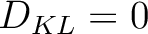 indicates that the two distributions are identical and no gain has been achieved upon seeing the data. In all of our examples, we report with respect to the input uniform prior distributions to the first inversion run.
Even though is generally unbounded, it is possible to compute a benchmark value for some simple case. For example, if we consider Gaussian prior and posterior distributions, the Kullback-Leibler divergence () can be expressed as
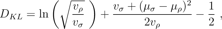 |
(10) |
 and
and  are the variance and mean of the distributions, respectively. It follows that if no information is gained during the inversion process and
 , then . If the standard deviation of the posterior reduces to half that of the prior with the same mean, the Kullback-Leibler divergence is equal to
 |
(11) |
|
|
|
|
Probabilistic moveout analysis by time warping |