|
|
|
|
A robust approach to time-to-depth conversion and interval velocity estimation from time migration in the presence of lateral velocity variations |
In a medium with a constant velocity gradient
It is easy to verify from equations 16 and 17 that
![]() ,
,
![]() and
and
![]() . Because there is no geometrical
spreading of image rays in this case, the Dix velocity will be equal to the interval velocity according to
equation 3. However, a Dix-inverted model will still be distorted if
. Because there is no geometrical
spreading of image rays in this case, the Dix velocity will be equal to the interval velocity according to
equation 3. However, a Dix-inverted model will still be distorted if ![]() because of the
lateral shift of image rays.
because of the
lateral shift of image rays.
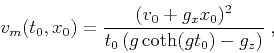
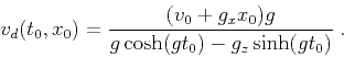
Figures 3 and 4 show a velocity model with
![]() km/s and
the corresponding analytical
km/s and
the corresponding analytical ![]() ,
, ![]() and
and ![]() . Clearly, the right domain boundary is
of in-flow type that violates our assumption. To address this challenge, we include Dix velocity
in regions beyond the original left and right boundaries during inversion, but mask out the cost in these regions.
It means that the time-to-depth conversion is performed in a sub-domain of time-domain attributes, such that
information on the in-flow boundary is available. Afterwards, we apply Dix inversion to the expanded model and
use the result as the prior model. We use the exact Dix velocity in equation 19
for evaluating the right-hand side of 5. Then, in total three linearization updates are carried
out, which decreases
. Clearly, the right domain boundary is
of in-flow type that violates our assumption. To address this challenge, we include Dix velocity
in regions beyond the original left and right boundaries during inversion, but mask out the cost in these regions.
It means that the time-to-depth conversion is performed in a sub-domain of time-domain attributes, such that
information on the in-flow boundary is available. Afterwards, we apply Dix inversion to the expanded model and
use the result as the prior model. We use the exact Dix velocity in equation 19
for evaluating the right-hand side of 5. Then, in total three linearization updates are carried
out, which decreases ![]() to relative
to relative ![]() . The radiuses of triangular smoother in shaping are
. The radiuses of triangular smoother in shaping are ![]() m
vertically and
m
vertically and ![]() m horizontally (
m horizontally (![]() m
m ![]()
![]() m). At last, we cut the computational domain back to its
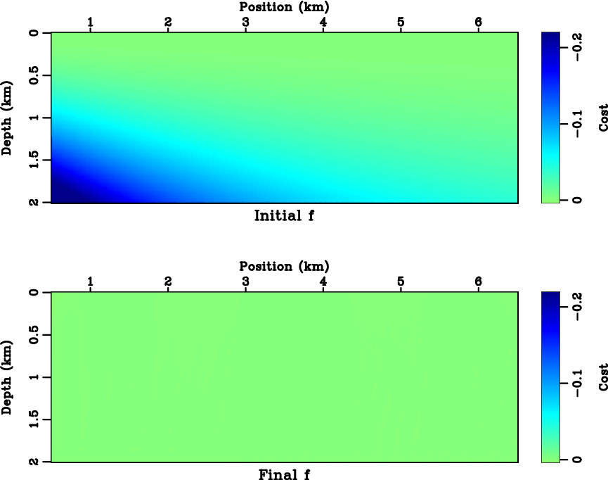
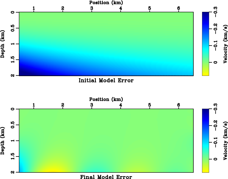
original size. Figures 5 and 6 compare the cost and model misfit before and after
inversion.
m). At last, we cut the computational domain back to its
original size. Figures 5 and 6 compare the cost and model misfit before and after
inversion.
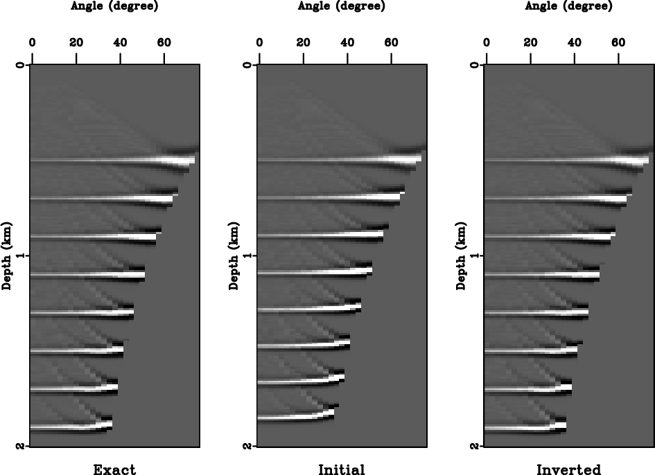
We also synthesize data with Kirchhoff modeling (Haddon and Buchen, 1981) for several horizontal reflectors using the exact model, and examine the subsurface scattering-angle common-image-gathers from Kirchhoff prestack depth migration (Xu et al., 2001) as an evidence of interval velocity improvements. In Figure 7, the shallower events do not improve significantly because the image rays have not yet bent considerably. Deeper events become noticeably flatter after applying the proposed method.
|
|---|
|
vgrad
Figure 3. (Top) a constant velocity gradient model and (bottom) the analytical Dix velocity |
|
|
|
|---|
|
analy
Figure 4. Analytical values of (top) |
|
|
|
|---|
|
cost
Figure 5. The cost defined by equation 9 (top) before and (bottom) after inversion. The least-squares norm of cost |
|
|
|
|---|
|
error
Figure 6. The difference between exact model and (top) initial model and (bottom) inverted model. The least-squares norm of model misfit is decreased from |
|
|
|
|---|
|
cigv
Figure 7. Comparison of the subsurface scattering-angle common-image-gathers at |
|
|
|
|
|
|
A robust approach to time-to-depth conversion and interval velocity estimation from time migration in the presence of lateral velocity variations |
![\begin{displaymath}
t_0 (z,x) = \frac{1}{g} \mathrm{arccosh} \left[ \frac{g^2 \l...
...^2 + g_x^2 z^2}
+ g_z z \right) - v g_z^2}{v g_x^2} \right]\;,
\end{displaymath}](img98.png)