|
|
|
|
A robust approach to time-to-depth conversion and interval velocity estimation from time migration in the presence of lateral velocity variations |
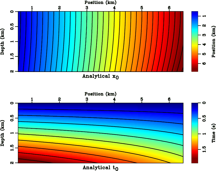
Another medium that provides analytical time-to-depth conversion formulas is
In Figure 8 we illustrate ![]() and
and ![]() in the model
in the model
![]()
![]() . To deal with the in-flow boundary issue, we apply the method described previously for
the constant velocity gradient example. Unlike equation 16, equation 21 indicates
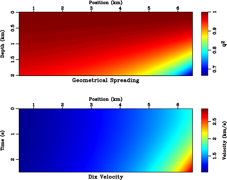
varying geometrical spreadings in the domain. Figure 9 shows the corresponding analytical
. To deal with the in-flow boundary issue, we apply the method described previously for
the constant velocity gradient example. Unlike equation 16, equation 21 indicates
varying geometrical spreadings in the domain. Figure 9 shows the corresponding analytical
![]() and
and ![]() . The geometrical spreading is significant at the lower-right corner of the domain,
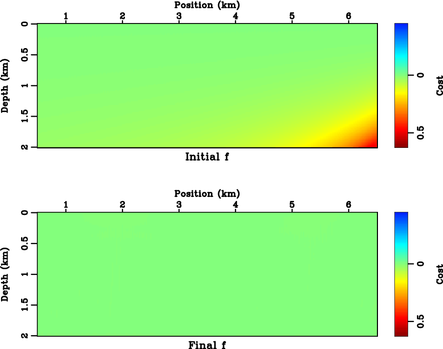
which translates to the cost at approximately the same location in Figure 10. We use analytical
Dix velocity as the input in the inversion. Starting from the Dix-inverted model and after three linearization
updates,
. The geometrical spreading is significant at the lower-right corner of the domain,
which translates to the cost at approximately the same location in Figure 10. We use analytical
Dix velocity as the input in the inversion. Starting from the Dix-inverted model and after three linearization
updates, ![]() decreases to relative
decreases to relative ![]() . The size of triangular smoother is
. The size of triangular smoother is ![]() m
m ![]()
![]() m.
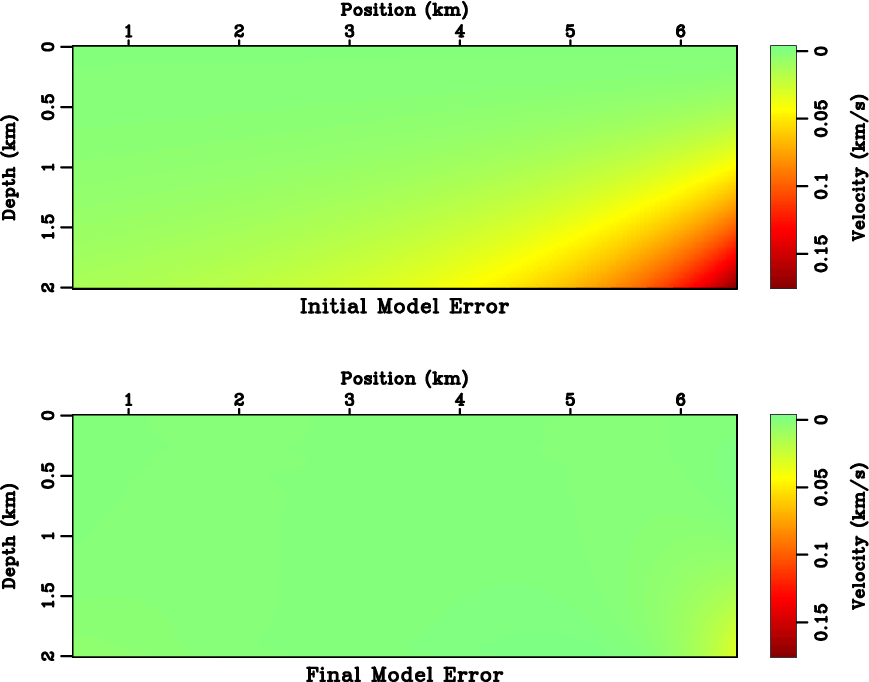
The model misfit, as demonstrated in Figure 11, is also improved.
m.
The model misfit, as demonstrated in Figure 11, is also improved.
|
|---|
|
hs2analy
Figure 8. Analytical values of (top) |
|
|
|
|---|
|
hs2grad
Figure 9. The (top) geometrical spreading and (bottom) Dix velocity associated with the model used in Figure 8. |
|
|
|
|---|
|
hs2cost
Figure 10. The cost (top) before and (bottom) after inversion. The least-squares norm of cost |
|
|
|
|---|
|
hs2error
Figure 11. The difference between exact model and (top) initial model and (bottom) inverted model. The least-squares norm of model misfit is decreased from |
|
|
|
|
|
|
A robust approach to time-to-depth conversion and interval velocity estimation from time migration in the presence of lateral velocity variations |
![\begin{displaymath}
t_0 (z,x) = \frac{\sqrt{2} z \left[ 2 w_0 - 4 q_x x + \sqrt{...
...qrt{(w_0 - 2 q_x x)^2 - 4 q_x^2 z^2} \right]^{\frac{1}{2}}}\;.
\end{displaymath}](img115.png)