A robust approach to time-to-depth conversion and interval velocity estimation from time migration in the presence of lateral velocity variations

The optimization formulation

Given boundary conditions 8, equation 6 describes the traveltime $t_0$ of a velocity model with a plane-wave source at the surface. For a given $t_0$, equation 7 is a first-order linear PDE on $x_0$ and thus computation of $x_0$ is straightforward. Our idea is inspired by a natural logic: if the resulting $x_0$ does not satisfy equation 5, we need to modify $v$ in a way such that the misfit decreases, and repeat the process until convergence.

Mathematically, we define a cost function $f (z,x)$ based on equation 5:

$$f (z,x) = \nabla x_0 \cdot \nabla x_0 - v_d^2 w\;,$$ (9)

where for convenience we use slowness-squared $w (z,x) = v^{-2} (z,x)$ instead of $v$. Note that $f$ is dimensionless. The discretized form of equation 9 reads

$$\mathbf{f} = (\nabla \mathbf{x_0} \cdot \nabla) \mathbf{x_0... ... - \mbox{diag}(\mathbf{v_d} \star \mathbf{v_d}) \mathbf{w}\;.$$ (10)

In equation 10, $\mathbf{f}, \mathbf{x_0}, \mathbf{v_d}$ and $\mathbf{w}$ are all column vectors after discretizing the computational domain $(z,x)$. For example, $\mathbf{x_0}$ is the discretized column vector of $x_0 (z,x)$. The vector $\mathbf{v_d}$ may require interpolation because it is in $(t_0,x_0)$ while the discretization is in $(z,x)$. The interpolation can be done after forward mapping from $(z,x)$ to $(t_0,x_0)$ at current velocity model. We denote an operator which is a matrix $\mathbf{L}_{x_0} = \nabla \mathbf{x_0} \cdot \nabla$. The other operator $\mbox{diag}()$ expands a vector into a diagonal matrix. Finally, the symbol $\star$ stands for an element-wise vector-vector multiplication.

As is common in many optimization problems, we seek to minimize the least-squares norm of $\mathbf{f}$:

$$E [\mathbf{w}] = \frac{1}{2} \Vert\mathbf{f}\Vert^2 = \frac{1}{2} \mathbf{f}^T \mathbf{f}\;,$$ (11)

where the superscript $T$ stands for transpose. The Gauss-Newton method in optimization requires linearizing the cost function in equation 10:

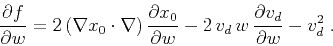$$\frac{\partial f}{\partial w} = 2 (\nabla x_0 \cdot \nabla... ...ial w} - 2 v_d w \frac{\partial v_d}{\partial w} - v_d^2\;.$$ (12)

The Fréchet derivative matrix $\mathbf{J}$ required by inversion is the discretized form of equation 12, i.e., $\mathbf{J} = \partial \mathbf{f} / \partial \mathbf{w}$. In Appendix B we find that $\mathbf{J}$ is a cascade and summation of several parts. An update $\delta \mathbf{w}$ at current $\mathbf{w}$ is found by solving the following normal equation arising from the Gauss-Newton approach (Björck, 1996):

$$\delta \mathbf{w} = \left[ \mathbf{J}^T \mathbf{J} \right]^{-1} \mathbf{J}^T (- \mathbf{f})\;.$$ (13)

Equations 11 and 13 together suggest a nonlinear inversion procedure for solving the original system of PDEs 5, 6 and 7. The inversion is analogous to traveltime tomography but with more complexity. The cost 9 can be interpreted as difference between modeled and observed geometrical spreadings. However, both of them depend on the model $v$, while in traveltime tomography the observed arrival times are independent of $v$. The forward modeling in our case involves two steps, which construct a curvilinear coordinate system that is sensitive to lateral velocity variations. On the other hand, the forward modeling in traveltime tomography consists of only one step. Last but not least, unlike traveltime tomography, we have observations everywhere in the computational domain, except for areas excluded due to instabilities of the numerical implementation, as we will discuss later.

Before introducing a numerical implementation, we would like to point out several important facts and assumptions that make a successful time-to-depth conversion possible by the proposed method:

• Caustics must be excluded from the computational domain. In regions where caustics develop, the gradient $\nabla x_0$ goes to infinity and the cost function is not well-defined. For all numerical examples in this paper, we do not encounter this issue. In the Discussion section, we provide a possible strategy to cope with this limitation.
• According to derivations in Appendix B, the calculation of $\delta \mathbf{w}$ depends on values of $\partial \mathbf{v_d} / \partial \mathbf{t_0}$ and $\partial \mathbf{v_d} / \partial \mathbf{x_0}$. Thus the input $v_d$ should be differentiable. This requirement can be satisfied during $v_m$ estimation by using regularization (Fomel, 2003).
• Similarly to all nonlinear inversions, the proposed method requires a prior model that is sufficiently close to desired model at the global minimum $E = 0$. Meanwhile, to guarantee stability and a smooth output, some form of regularization should be imposed during inversion (Zhdanov, 2002; Engl et al., 1996).
• Our formulation does not change the ill-posed nature of the original problem. One assumption is that condition 8 describes all in-flow domain boundaries of $t_0$ and $x_0$. In other words, the image rays are only allowed to be either parallel to or exiting (out-flow) all other boundaries of the computational domain except the surface.

For the prior model, we adopt the Dix-inverted model. In other words, we seek to refine the interval velocity given by equation 2 by taking the geometrical spreading of image rays into consideration according to equation 3.

A robust approach to time-to-depth conversion and interval velocity estimation from time migration in the presence of lateral velocity variations