Stratigraphic coordinates, a coordinate system tailored to seismic interpretation

Examples of Stratigraphic coordinates

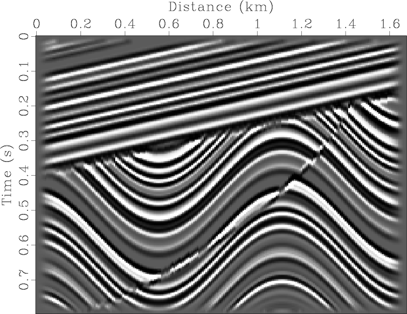
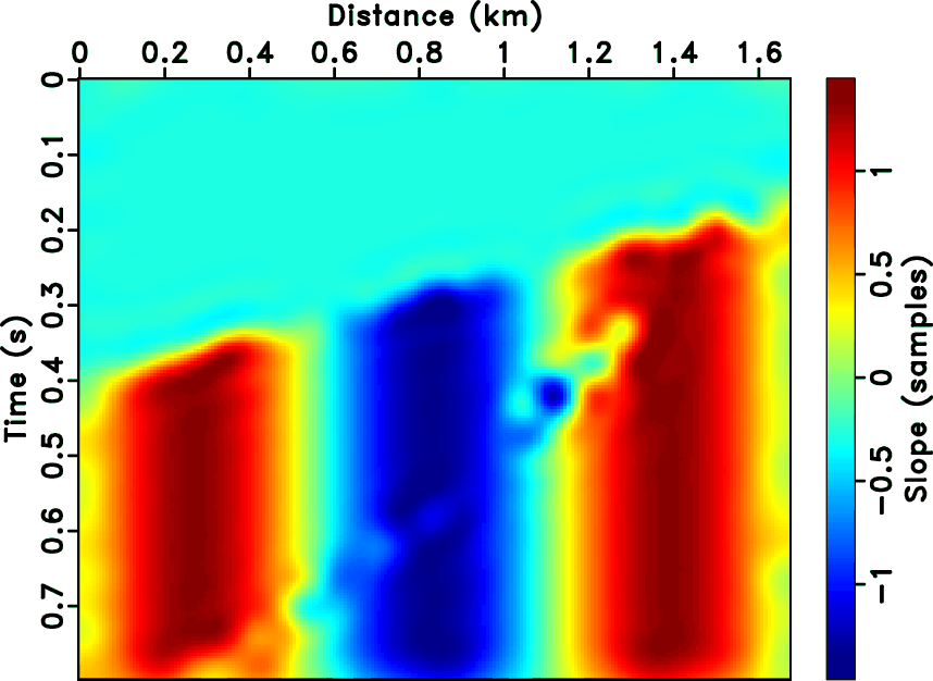
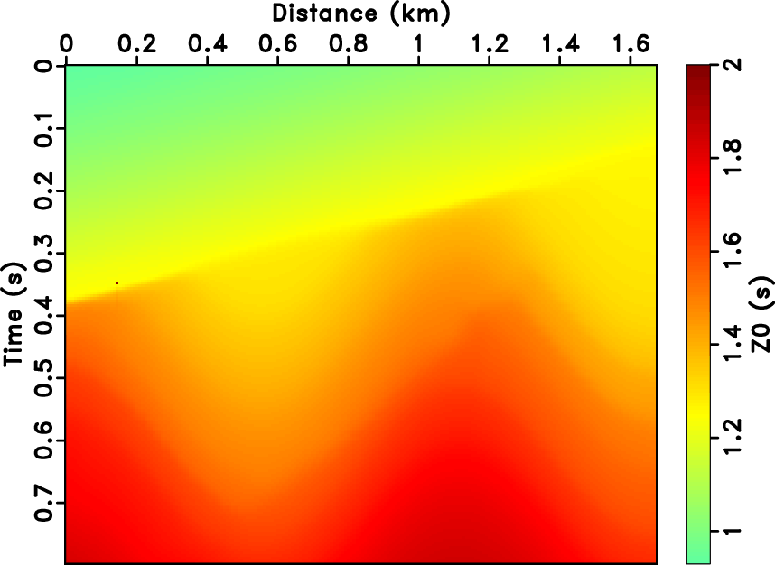
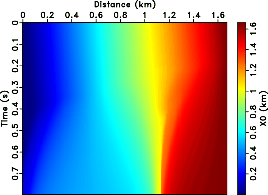
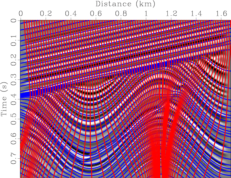
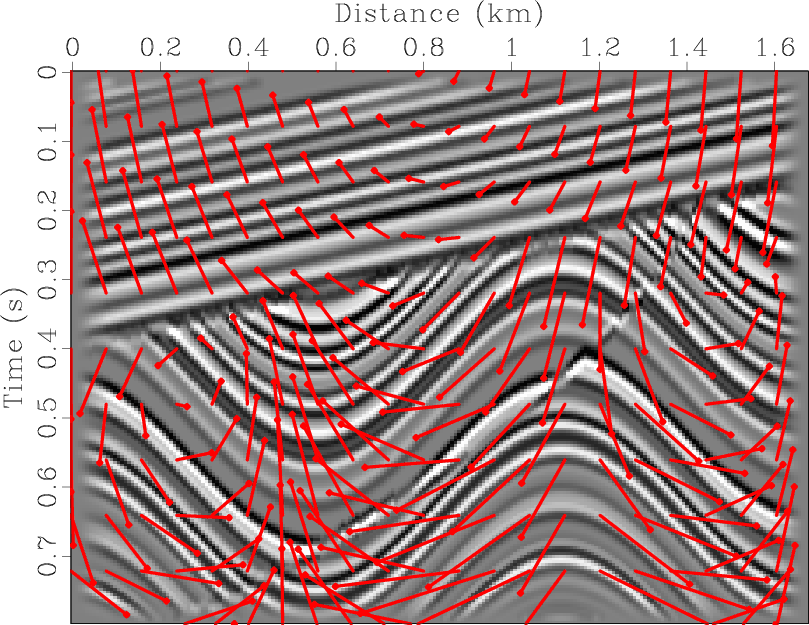
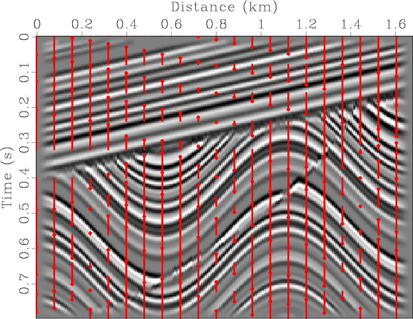
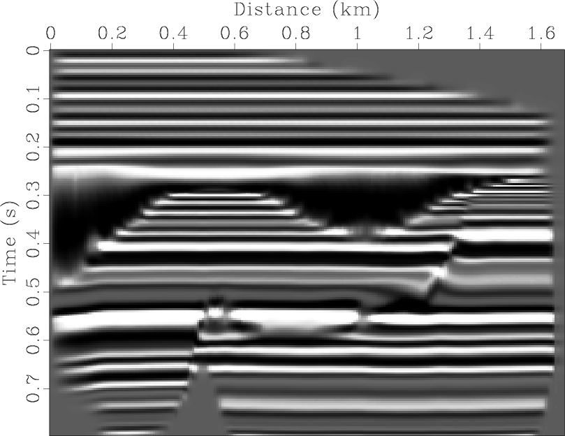
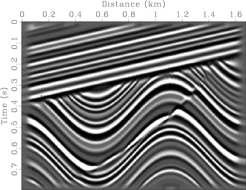
For a simple illustration of stratigraphic coordinates, we use a 2D synthetic seismic image from Claerbout (2006), which contains layers with sinusoidal dip variations, faulted and truncated by an unconformity, and dipping beds with constant slope above the unconformity (Figure 1a). Figure 1b shows local slopes measured by plane-wave destruction and delineates the slope field variation. Figure 2a shows automatically picked horizons obtained by the predictive-painting algorithm. After solving the gradient equation 1, we acquire the other axis of the stratigraphic coordinate system (Figure 2b). Figure 3a shows the stratigraphic coordinates grid overlain on the regular Cartesian coordinates of the seismic image. Complex tectonic deformations expressed in faults and folds cannot in general be undone by a simple vertical stretch and squeeze operator. In contrast, the transformation to stratigraphic coordinates allows for complex displacements, which can better capture and thus undo non-trivial tectonic deformations. Arrows in Figure 3b show the amount and direction of shift that it takes for different samples to be transformed from their original position in the seismic image to their corresponding positions in the flattened image through the stratigraphic coordinates algorithm. For comparison, arrows in Figure 3c represent how different samples shift under conventional flattening methods. The seismic image gets flattened when the data from the regular coordinate system are transferred to stratigraphic coordinates. The result is shown in Figure 4a. Apart from the structural (fault) and stratigraphic (erosional truncation) discontinuities, the input image is successfully flattened. Figure 4b shows that by returning from stratigraphic coordinates to regular coordinates, one can recostruct the features of the original image effectively.

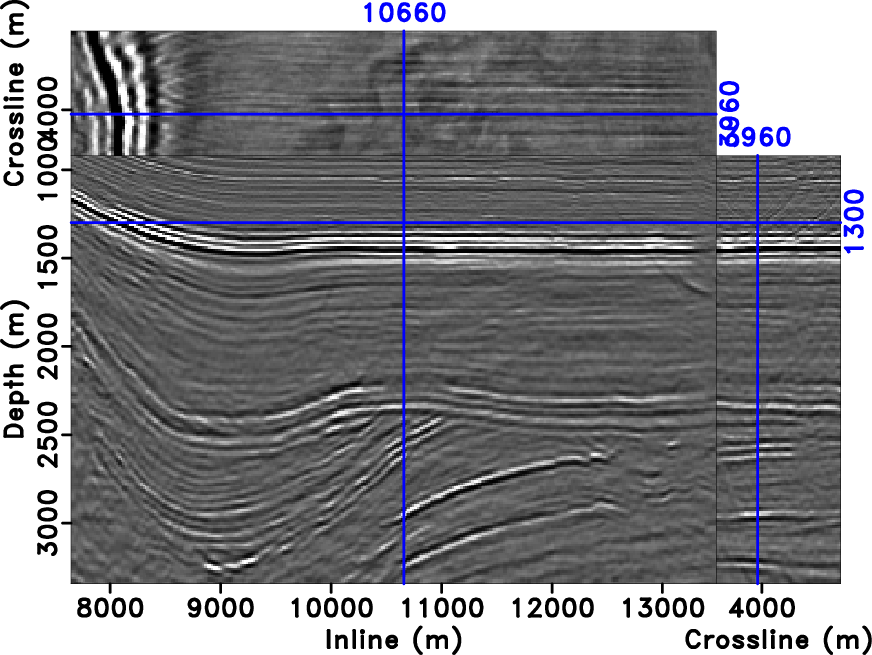
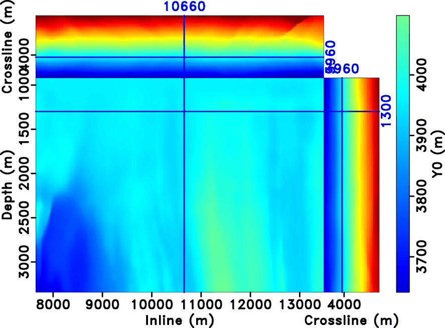
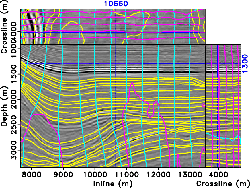
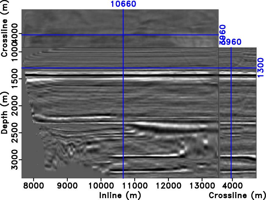
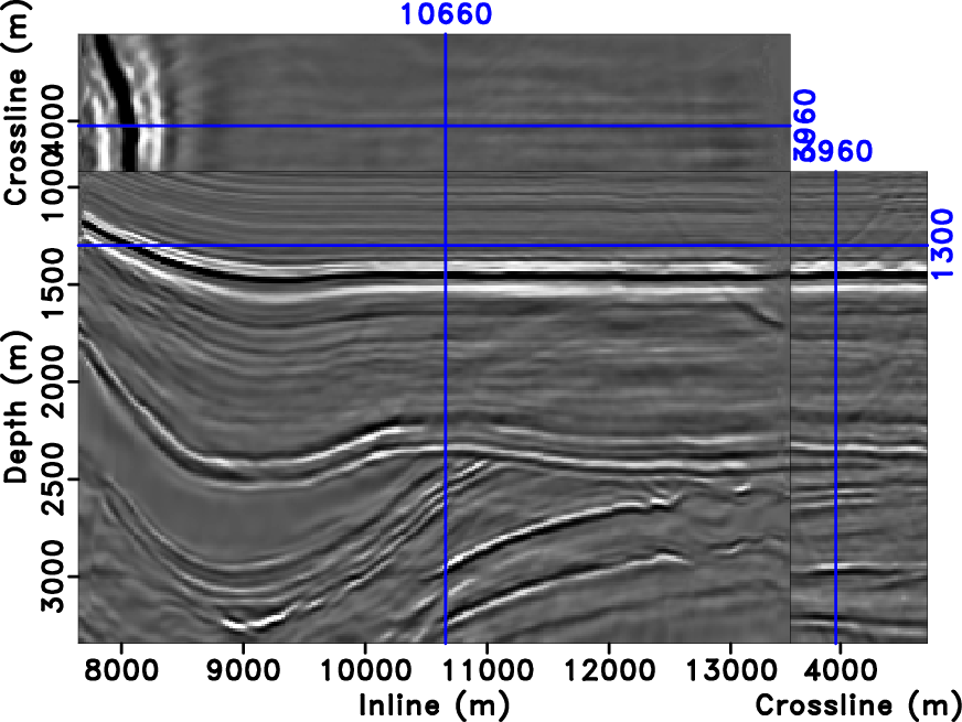
Figure 5a shows the input image for a field-data test reproduced from Lomask et al. (2006) and Fomel (2010). The input is a depth-migrated 3-D image with structural folding and angular unconformities. The three axes of the stratigraphic coordinates are shown in Figure 6. Figure 7a displays the image in the regular Cartesian coordinates overlain by its stratigraphic coordinates grid. The flattened image in the stratigraphic coordinate system, shown in Figure 7b, can be transferred back to the regular Cartesian coordinates to reconstruct the original image (Figure 7c).

sigmoid,sdip
Figure 1. (a) Synthetic seismic image from Claerbout (2006). (b) Local slopes measured by plane-wave destruction.

t0sig,x0sig
Figure 2. (a) First axis ($Z_0$) of stratigraphic coordinates in the regular coordinates obtained by predictive painting. (b) Second axis ($X_0$) of the stratigraphic coordinate system acquired by solving the gradient equation (equation 1).

sigmoid-t0sigx0sig,shift,shift0
Figure 3. (a) Two axes of the stratigraphic coordinate system relative to the regular coordinate system. The synthetic image with corresponding shift represented by red arrows through using stratigraphic coordinates (b) and conventional flattening methods (c).

sigmoid2,sigmoid1
Figure 4. (a) Synthetic image from Figure 1a flattened by transferring the image to the stratigraphic coordinate system. (b) Unflattened synthetic image reconstruction by returning from stratigraphic coordinates to regular coordinates.

win,wdip1,wdip2
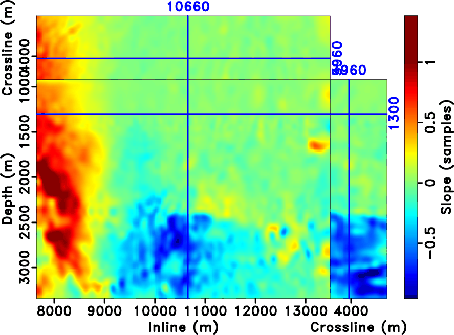
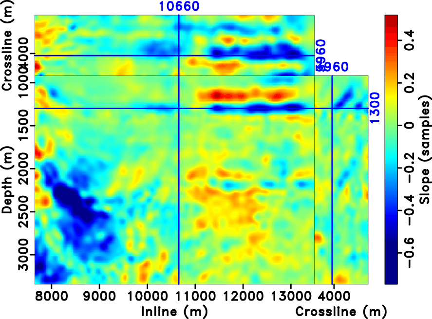
Figure 5. (a) North Sea image from Lomask et al. (2006) and its inline (b) and cross-line (c) slopes estimated by plane-wave destruction.

t0real1,x0real1,y0real2
Figure 6. (a) First axis ($Z_0$), (b) second axis ($X_0$), and (c) third axis ($Y_0$) of stratigraphic coordinates in the North Sea image.

coord,win1,win2
Figure 7. (a) Three axes of stratigraphic coordinates of Figure 5a plotted as a grid in their Cartesian coordinates. (b) North Sea image after flattening (transferring image to stratigraphic coordinates). (c) North Sea image reconstruction by returning from stratigraphic coordinates to regular coordinates.

Stratigraphic coordinates, a coordinate system tailored to seismic interpretation