|
|
|
|
Full waveform inversion of passive seismic data for sources and velocities |
Next: Numerical examples Up: Theory Previous: Sparse weighting function
|
|
|
|
Full waveform inversion of passive seismic data for sources and velocities |
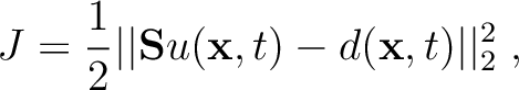
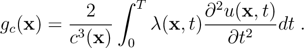
 norm:
where
norm:
where
 is the wavefield,
 is the observed seismic data and
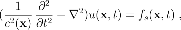
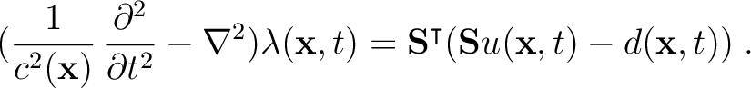
 is the matrix that defines aquisition geometry. The corresponding state and adjoint state equations can be expressed as
where
is the matrix that defines aquisition geometry. The corresponding state and adjoint state equations can be expressed as
where
 is the adjoint wavefield,
 is the velocity and
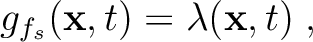
 is the source function . The gradients for source and velocity are respectively:
Note that the gradient with respect to the seismic source is exactly the adjoint wavefield, i.e., the time-reversal wavefield modeled by the adjoint state equation. This explains why the conventional time-reversal imaging methods are appropriate for locating seismic sources. However, the difference between the true seismic source and a time-reversal wavefield is quite significant. First, the true seismic source
is sparse, while a time-reversal wavefield is not. Second, even at locations and times that correspond to true seismic sources, the time-reversal wavefield does not provide accurate amplitude and phase information.
is the source function . The gradients for source and velocity are respectively:
Note that the gradient with respect to the seismic source is exactly the adjoint wavefield, i.e., the time-reversal wavefield modeled by the adjoint state equation. This explains why the conventional time-reversal imaging methods are appropriate for locating seismic sources. However, the difference between the true seismic source and a time-reversal wavefield is quite significant. First, the true seismic source
is sparse, while a time-reversal wavefield is not. Second, even at locations and times that correspond to true seismic sources, the time-reversal wavefield does not provide accurate amplitude and phase information.
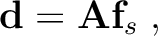
To address this issue, we note that the wavefield is linearly dependent on the source term (Rickett, 2013). Rewriting equation 8 as a linear operator:
where linear operator represents the combination of acoustic wave equation and acquisition geometry matrix
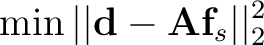
. Given a starting velocity model, one can obtain accurate information about the source by solving the least-squares problem
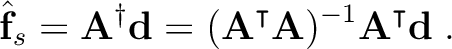
using the pseudo-inverse
In the rest part of the paper, we will refer to the method defined by equation 14 as least-squares time-reversal imaging (LSTRI). Although LSTRI is a linear inversion, we recognize that the model space is actually four-dimensional, and includes the three spatial axes and one time axis. Without proper preconditioning, the computational cost of such an inversion can be impractical. We propose to use the weighting function derived in equation 5 as a diagonal model weighting matrix to precondition the conjugate gradient (CG) iterations. Since
represents the combination of acoustic wave equation and acquisition geometry matrix
. Given a starting velocity model, one can obtain accurate information about the source by solving the least-squares problem
using the pseudo-inverse
In the rest part of the paper, we will refer to the method defined by equation 14 as least-squares time-reversal imaging (LSTRI). Although LSTRI is a linear inversion, we recognize that the model space is actually four-dimensional, and includes the three spatial axes and one time axis. Without proper preconditioning, the computational cost of such an inversion can be impractical. We propose to use the weighting function derived in equation 5 as a diagonal model weighting matrix to precondition the conjugate gradient (CG) iterations. Since
 effectively restricts CG to only update the locations that correspond to possible source locations, the eigenvalues of the matrix being inverted become better clustered and CG is able to achieve a faster convergence rate (Shewchuk, 1994).
The starting velocity model used to invert for the passive sources might be inaccurate. Most often, they are derived from well logs or travel-time tomography. FWI is capable of providing more detailed velocity structures. After initial source inversion, the inverted source can be used in FWI to update the velocity. Furthermore, one can jointly update the source and velcoty under the framework of the variable projection method (Aravkin et al., 2012; Golub and Pereyra, 1973; Rickett, 2013). In practice, we perform sufficient linear iterations to obtain accurate source functions and only a few nonlinear iterations to update the velocity model in an alternating fashion.
|
|
|
|
Full waveform inversion of passive seismic data for sources and velocities |