Numerical examples

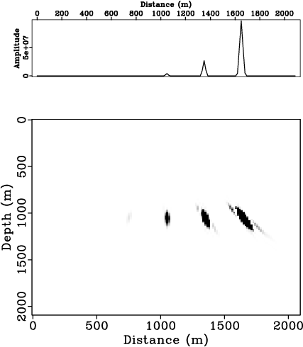
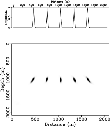
In our first example, we test the effectiveness of the local normalization operator in balancing the amplitudes of passive sources of different magnitudes. We use a vertical gradient velocity model with five sources at the same depth but with increasing magnitudes. Using HCTRI with ten groups of receivers, only three events with the highest magnitudes are identifiable from the stacked image (Figure 1a). After local normalization, the amplitude of all source images get normalized to one, which makes them fully identifiable after stacking (Figure 1b).

location0,location-new
Figure 1. (a) Source location calculated by HCTRI using ten groups of receivers. The amplitude is highly unbalanced due to the multiplication process. (b) Local normalized HCTRI image. The amplitude of all the sources are successfully normalized to one. The top panels demonstrates a trace cutting horizontally through the imaged hypocenters.

Next, we test the improved convergence rate of the preconditioned LSTRI using CG iterations. In a smoothly varying synthetic velocity model, three sources of varying magnitudes were excited at delayed times (Figure 2a). The recorded data contain three events of varying amplitudes and arrival times (Figure 2). The data misfit of LSTRI after $10$ iterations shows significant residual energy compared with LSTRI with the proposed preconditioning after $10$ iterations. The normalized source signature extracted from the true source location demonstrates that the preconditioned LSTRI provides the best estimation of the true source signature, compared with TRI and LSTRI. The convergence rate measured by normalized data misfit shows that the proposed preconditioning dramatically speeds up the convergence rate (Figure 4).

sov,data,res-inv1,res-inv2
Figure 2. (a)A vertical gradient velocity with three passive sources of variable magnitudes. (b) Synthetic passive data recorded by a surface array. Three events have been recorded. (c) Data misfit produced by LSTRI after $10$ iterations. (d) Data misfit produced by preconditioned LSTRI after $10$ iterations. Plotting clip are kept the same for all three cases.

src-traces,src-tr-traces,inv1-traces,inv2-traces
Figure 3. Normalized source signature of (a) true passive source; (b) passive source estimated by TRI; (c) passive source estimated by LSTRI after $10$ iterations; (d) passive source estimated by preconditioned LSTRI after $10$ iterations.

conv
Figure 4. The convergence rate of LSTRI and preconditioned LSTRI. The dashed line denotes regular LSTRI, and the solid line denotes preconditioned LSTRI.

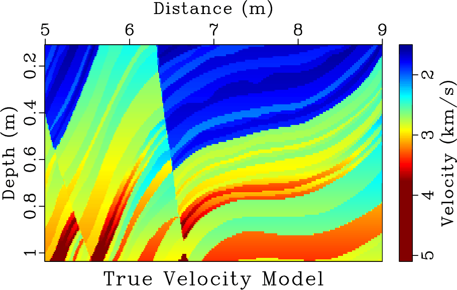
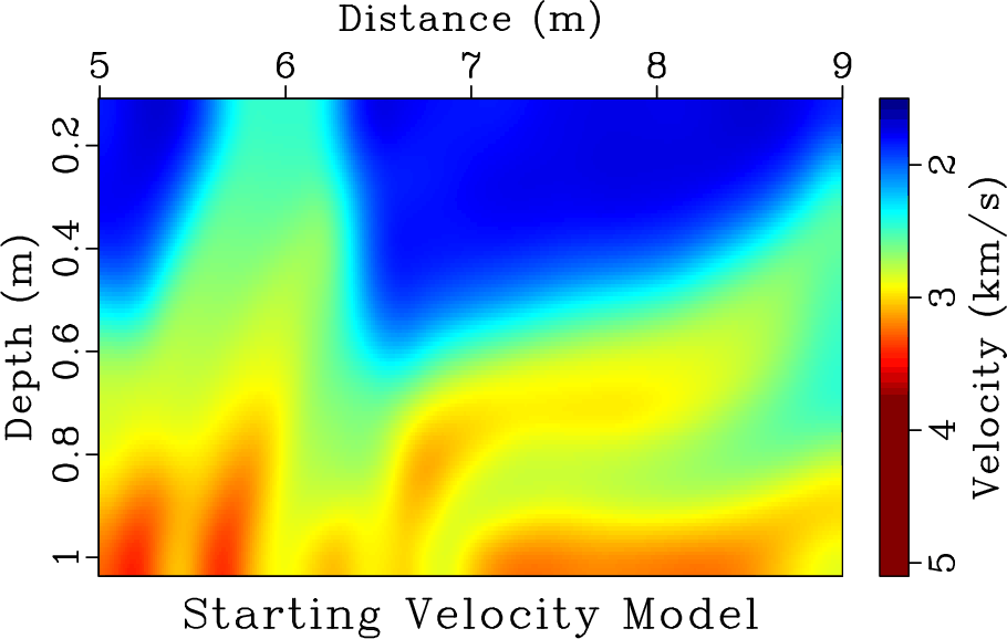
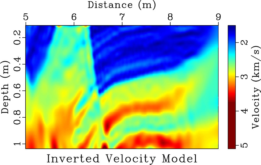
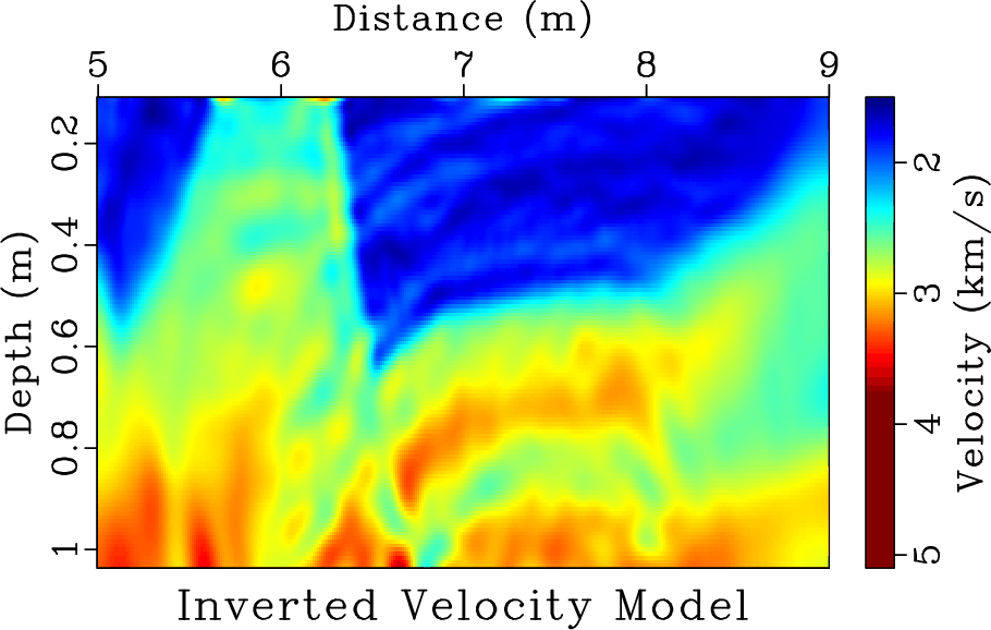
Finally, we combine the preconditioned LSTRI with acoustic FWI using the variable projection method and apply it to a synthetic example. Three stages of passive seismic events were recorded, each containing six events. The starting velocity model (Figure 5b) is a smoothed version of the real one (Figure 5a). A total of $60$ nonlinear iterations were performed for two FWI experiments. The first experiment is conventional FWI using an inverted source based on the true velocity model (Figure 5c). The second experiment uses the variable projection method to jointly invert for both passive sources and the velocity model (Figure 5d). Both experiments produce reasonable velocity updates, especially at high wavenumbers. The footprints of passive sources are visible in both inverted models. FWI with a known source was able to recover more detailed features in the velocity model compared with FWI with unknown sources using variable projection and the same number of iteraitons. It is reasonable to expect the joint inversion process to suffer from a slower convergence rate compared with that of the simpler task of inverting for velocity alone.

vel,vel-start,vel-inv-only,vel-inv-joint
Figure 5. (a) True velocity model; (b) starting velocity model; (c) inverted model using the known source after $60$ iterations; (d) inverted model using the variable projection method after $60$ iterations.