|
|
|
|
Diffraction imaging and time-migration velocity analysis using oriented velocity continuation |
Conventional velocity analysis resolution suffers in this dataset from the limitations
imposed by the depth of a seabed in the area (average of
![]() )
and a relatively short
)
and a relatively short ![]() streamer length. For deep water datasets
diffractions may exhibit better illumination than reflections because
diffraction aperture is not restricted to the recording array length, enabling them to provide a potentially more detailed velocity distribution. This behavior makes OVC migration velocity
analysis appealing.
streamer length. For deep water datasets
diffractions may exhibit better illumination than reflections because
diffraction aperture is not restricted to the recording array length, enabling them to provide a potentially more detailed velocity distribution. This behavior makes OVC migration velocity
analysis appealing.
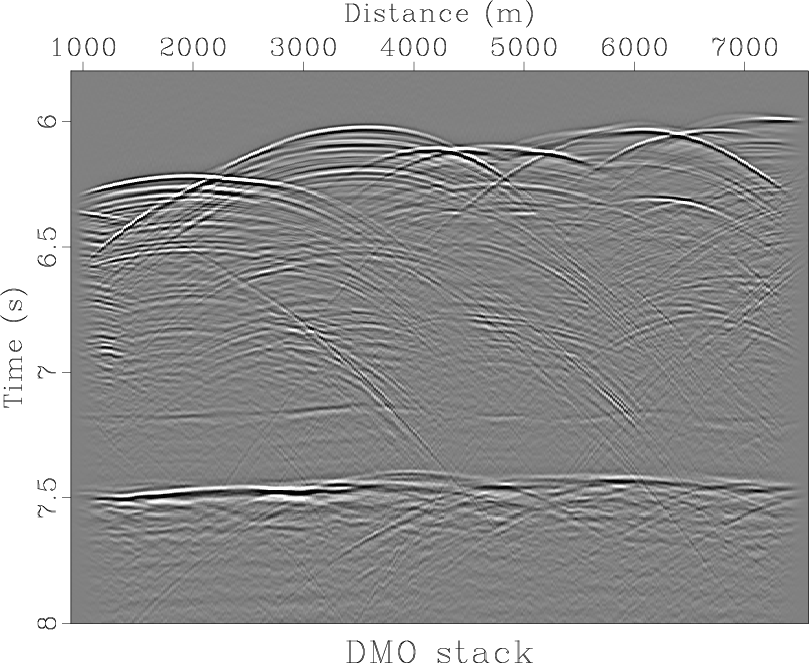
The DMO stacked section considered in this study is shown in Figure 10.
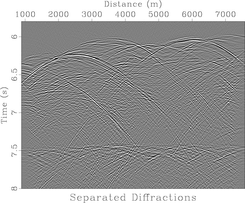
Diffractions are extracted via plane-wave destruction (Figure 11),
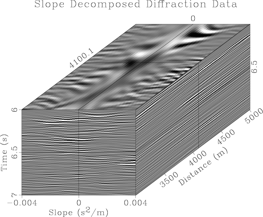
warped to squared time, and decomposed into slope.
Figure 12 shows slope decomposed data warped back to regular
time for ease of comparison with slope decomposed images appearing later.
Next, we take the decomposed data through oriented velocity
continuation over a range of sixty constant migration velocities beginning
with
![]() using a
using a
![]() step.
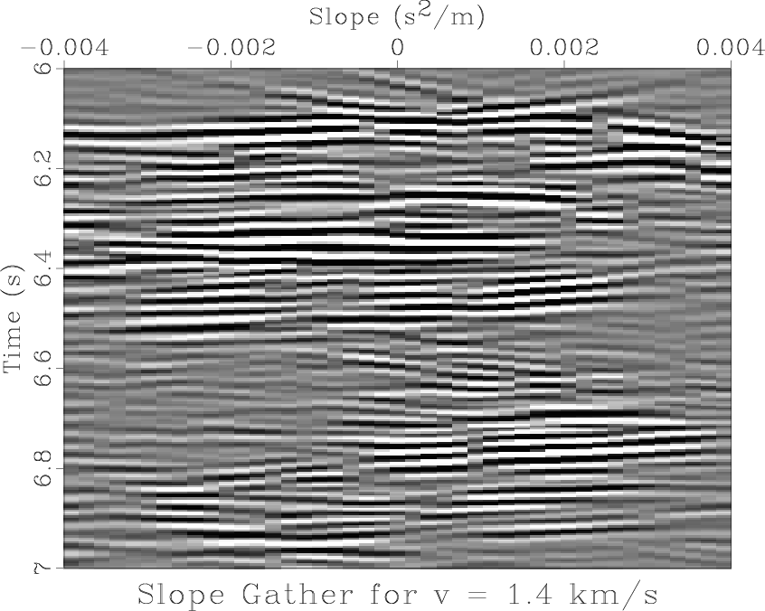
Diffraction events bend upward in the slope gather centered above
step.
Diffraction events bend upward in the slope gather centered above ![]() with the minimum tested migration velocity (Figure 14a), indicating under-migration.
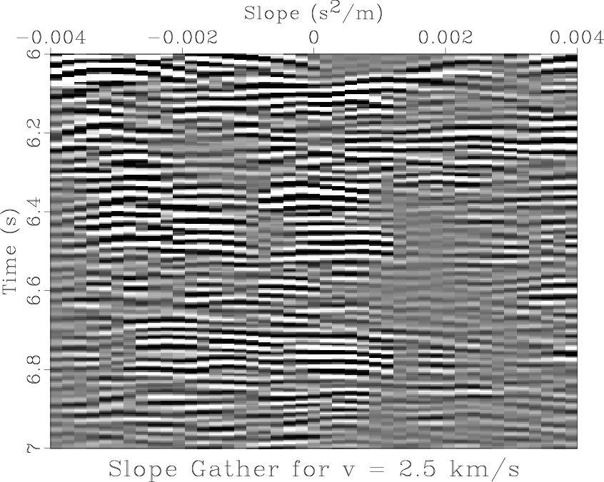
Diffraction events in the slope gather centered above the same location with the maximum
tested migration velocity (Figure 14b) bend downward, indicating over-migration.
with the minimum tested migration velocity (Figure 14a), indicating under-migration.
Diffraction events in the slope gather centered above the same location with the maximum
tested migration velocity (Figure 14b) bend downward, indicating over-migration.
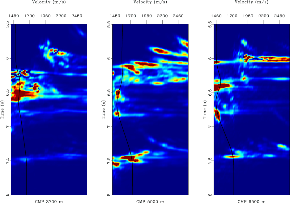
Gather semblance is calculated for each continuation velocity, and migration velocity
is automatically picked by attempting to maximize semblance for plausible velocity values
at each CMP location.
Semblance panels with superimposed picks are shown
in Figure 15.
Anomalies corresponding to higher velocities than
the picked trend may correspond to reflections
with high curvature, like the one located between ![]() and
and ![]() between
between ![]() and
and ![]() in Figures 10 and 11. Highly curved reflections
have a similar behavior to diffractions in response to migration velocity perturbation (Sava et al., 2005), but focus at a higher velocity than the correct one.
Intersection of over-migrated reflection and diffraction
tails from the rugose seabed, some of which are out of plane, leads to
diffraction-like events, another cause of false semblance highs. These are visible in the
three semblance panels of Figure 15 above
in Figures 10 and 11. Highly curved reflections
have a similar behavior to diffractions in response to migration velocity perturbation (Sava et al., 2005), but focus at a higher velocity than the correct one.
Intersection of over-migrated reflection and diffraction
tails from the rugose seabed, some of which are out of plane, leads to
diffraction-like events, another cause of false semblance highs. These are visible in the
three semblance panels of Figure 15 above ![]() . Low velocity semblance
anomalies corresponding to the flattening of out of plane diffractions are also visible in the
middle interval of the semblance panels, particularly near
. Low velocity semblance
anomalies corresponding to the flattening of out of plane diffractions are also visible in the
middle interval of the semblance panels, particularly near
![]() in the central and
right panels centered above
in the central and
right panels centered above ![]() and
and ![]() .
.
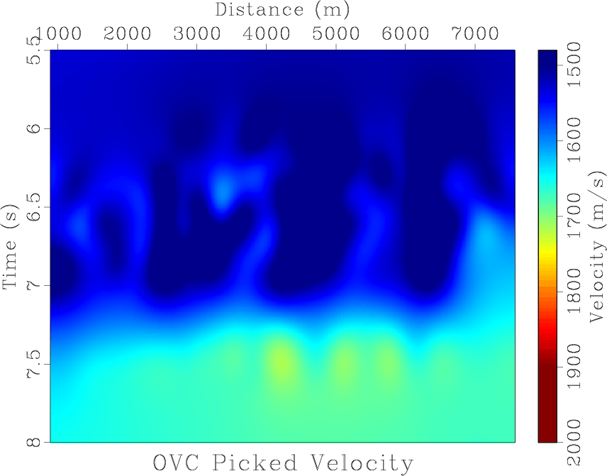
Combining the semblance velocity picks from each CMP provides a time-migration velocity field, shown in Figure 16. As noted above, several anomalously low velocity zones exist in the picked field, primarily between ![]() and
and ![]() where the attempted flattening of out of plane diffractions leads to a low picked velocity.
where the attempted flattening of out of plane diffractions leads to a low picked velocity.
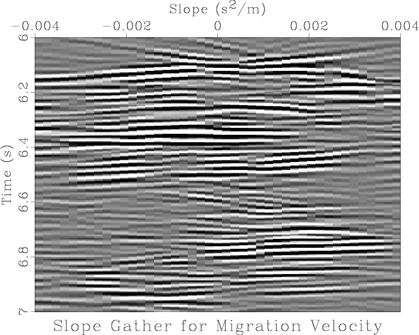
Gathers corresponding to the picked velocity are selected. Examining a slope gather
from ![]() generated using the picked migration velocity (Figure 14c), diffraction events now appear flat, particularly the one located near
generated using the picked migration velocity (Figure 14c), diffraction events now appear flat, particularly the one located near ![]() , indicating that they have been correctly migrated.
, indicating that they have been correctly migrated.
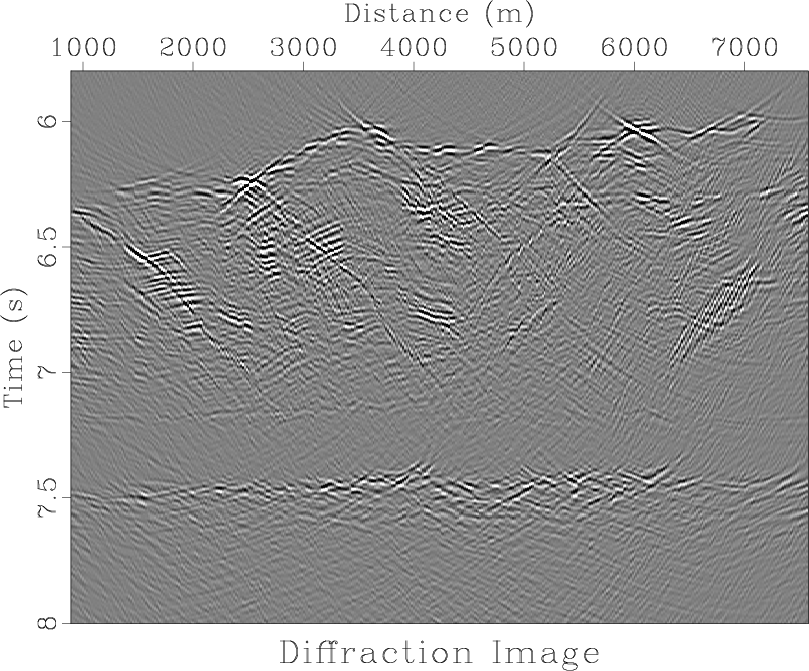
Stacking gathers generated from the the picked velocity over slope provides the
diffraction image in Figure 17. We apply oriented velocity continuation
to the DMO stacked data from Figure 10 and stack over gathers
selected with the appropriate velocity to generate the image of reflections and diffractions in
Figure 18. Both images highlight fault surfaces.
Finer discontinuities, such as those associated with the rough surface of the subducting plate crust, located near
![]() (Moore and Shipley, 1993), are more prominent on the diffraction image and tend to be well focused, supporting the accuracy of the picked velocity.
(Moore and Shipley, 1993), are more prominent on the diffraction image and tend to be well focused, supporting the accuracy of the picked velocity.
|
|---|
|
slice
Figure 10. Nankai DMO stacked section. |
|
|
|
|---|
|
dif
Figure 11. Nankai separated diffractions. |
|
|
|
|---|
|
tpx
Figure 12. Slope decomposition of Nankai diffraction data |
|
|
|
|---|
|
txp-migrated
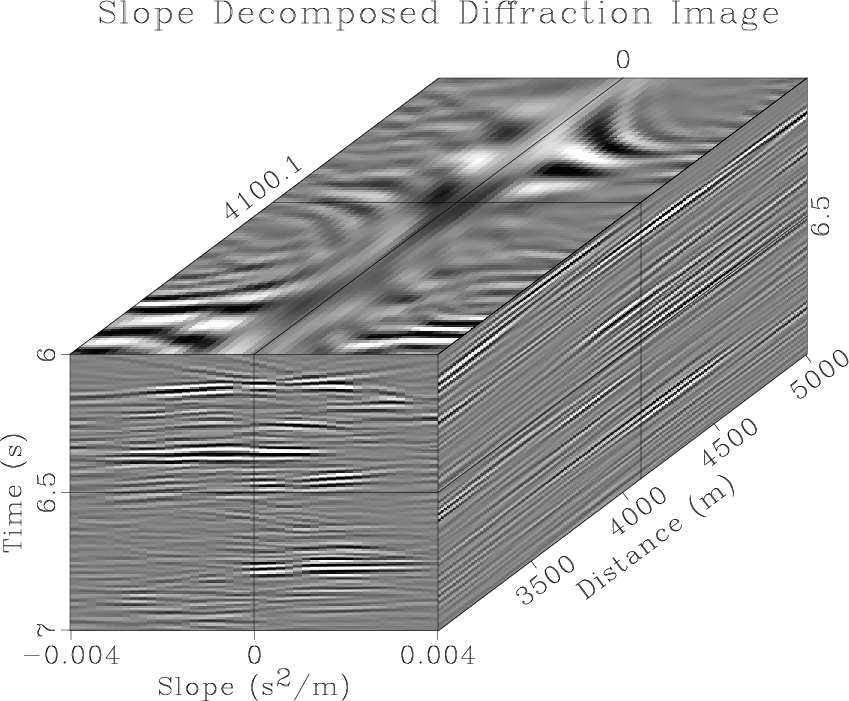
Figure 13. Slope decomposition of Nankai diffraction image |
|
|
|
|---|
|
txp14-slice-center-s,txp25-slice-center-s,txp-slice-center-s
Figure 14. Slope gathers centered above |
|
|
|
|---|
|
g-picking
Figure 15. Velocity scan semblance panels with superimposed picks from left to right for CMPs at |
|
|
|
|---|
|
vpick-semb
Figure 16. Velocity picked from slope-gather flattening |
|
|
|
|---|
|
vc-slice-semb
Figure 17. Diffraction image generated with the velocity from the Figure 16. |
|
|

|
|---|
|
vc-fw-slice-semb
Figure 18. Conventional image generated with the velocity from the Figure 16. |
|
|
|
|
|
|
Diffraction imaging and time-migration velocity analysis using oriented velocity continuation |