|
|
|
|
Random noise attenuation by |
In this section, we first reuse the previously discussed synthetic data (Figure 1(j)), then show two other synthetic data and one field data example to demonstrate the performance of ![]() EMDPF.
EMDPF.
Figure 1(k) shows the denoised result after ![]() EMDPF. The removed noise section is shown in Figure 1(l).
Comparing Figure 1(i) and Figure 1(l), we see that the useful events leaked into Figure 1(i) have been returned to the denoised result (Figure 1(k)), while the noise level stays nearly unchanged.
EMDPF. The removed noise section is shown in Figure 1(l).
Comparing Figure 1(i) and Figure 1(l), we see that the useful events leaked into Figure 1(i) have been returned to the denoised result (Figure 1(k)), while the noise level stays nearly unchanged.
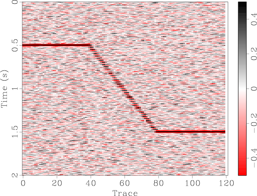
The second synthetic example is composed of one linear dipping event and two flat events (Figure 4). A 40 Hz Ricker wavelet has been used with a time sample interval of 4 ms. The number of samples for each trace is 501, and the number of traces is 120. Figures 4(d), 4(e), and 4(f) illustrate the comparison of denoised results of the synthetic data using ![]() predictive filtering,
predictive filtering, ![]() EMD filtering, and
EMD filtering, and ![]() EMDPF, respectively. Figure 4(a) is the noise free data, Figure 4(b) is Gaussian white noise, and Figure 4(c) is the noisy data. The SNR of the noisy data is 2.0 (using the previous definition of SNR). Figures 4(g), 4(h), and 4(i) show the removed noise sections corresponding to
EMDPF, respectively. Figure 4(a) is the noise free data, Figure 4(b) is Gaussian white noise, and Figure 4(c) is the noisy data. The SNR of the noisy data is 2.0 (using the previous definition of SNR). Figures 4(g), 4(h), and 4(i) show the removed noise sections corresponding to ![]() predictive filtering,
predictive filtering, ![]() EMD, and
EMD, and ![]() EMDPF, respectively. From Figure 4(g), we can see that
EMDPF, respectively. From Figure 4(g), we can see that ![]() predictive filtering harms both flat and dipping events to some extent. Although by increasing the length of the predictive step we can decrease the damage done to the signals, the noise suppression is less effective because of the stronger prediction of noise. Also, as seen in Figure 4(d), the
predictive filtering harms both flat and dipping events to some extent. Although by increasing the length of the predictive step we can decrease the damage done to the signals, the noise suppression is less effective because of the stronger prediction of noise. Also, as seen in Figure 4(d), the ![]() predictive filtering introduces some artefacts. In Figure 4(h), we see that
predictive filtering introduces some artefacts. In Figure 4(h), we see that ![]() EMD tends to harm much of the dip energy but preserves entirely the flat events. Using the same predictive filtering parameters, we see from Figure 4(i) that both flat and dipping signals are hardly affected when
EMD tends to harm much of the dip energy but preserves entirely the flat events. Using the same predictive filtering parameters, we see from Figure 4(i) that both flat and dipping signals are hardly affected when ![]() EMDPF is applied. In this example, the first IMF is removed for prediction in the process of
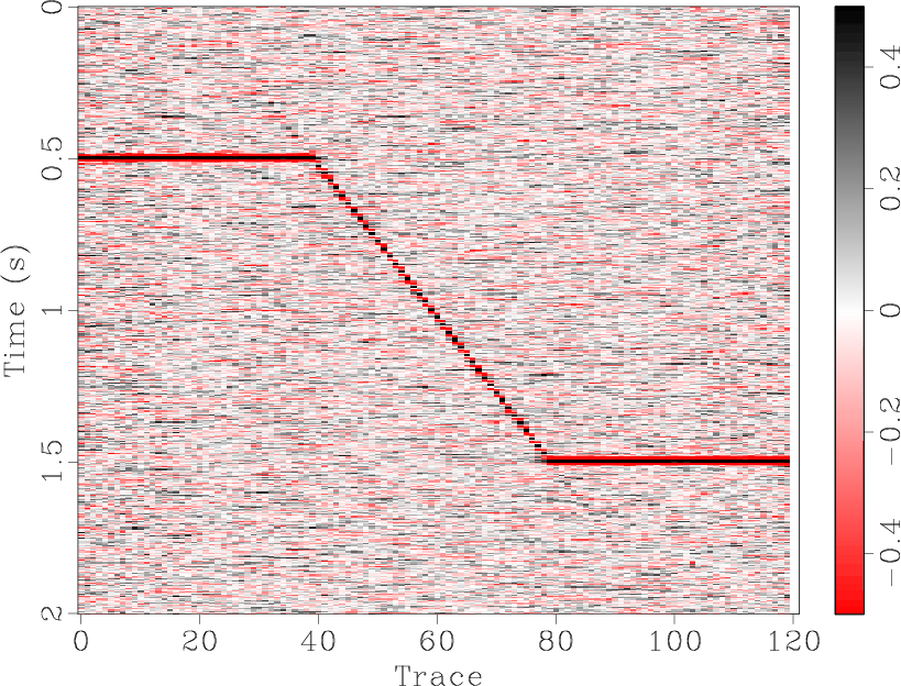
EMDPF is applied. In this example, the first IMF is removed for prediction in the process of ![]() EMDPF. Figure 5 demonstrates the sensitivity of the
EMDPF. Figure 5 demonstrates the sensitivity of the ![]() EMDPF for increasing the number of filtered IMFs. We can see that, as the number of filtered IMFs increases, the denoising result becomes more similar to
EMDPF for increasing the number of filtered IMFs. We can see that, as the number of filtered IMFs increases, the denoising result becomes more similar to ![]() predictive filtering; that is, more noise is removed and more obvious artefacts appear in the denoised section. However, for
predictive filtering; that is, more noise is removed and more obvious artefacts appear in the denoised section. However, for ![]() EMDPF, the horizontal events are always totally preserved, which supposes a generally better denoising result than
EMDPF, the horizontal events are always totally preserved, which supposes a generally better denoising result than ![]() predictive filtering.
predictive filtering.


|
|---|
|
syn02-clean,syn02-noise,syn02,syn02-fxdecon,syn02-fxemd,syn02-fxemdpf,syn02-fxdecon-noise,syn02-fxemd-noise,syn02-fxemdpf-noise
Figure 4. Comparison of denoising effects. (a) Clean data. (b) Gaussian white noise. (c) Noisy data. (d) Denoised result by |
|
|


|
|---|
|
syn02-fxemdpf-1imf,syn02-fxemdpf-1imf-noise,syn02-fxemdpf-2imf,syn02-fxemdpf-2imf-noise,syn02-fxemdpf-3imf,syn02-fxemdpf-3imf-noise
Figure 5. Comparison of denoising effects. (a) |
|
|


|
|---|
|
syn03-clean,syn03-noise,syn03,syn03-fxdecon,syn03-fxemd,syn03-fxemdpf,syn03-fxdecon-noise,syn03-fxemd-noise,syn03-fxemdpf-noise
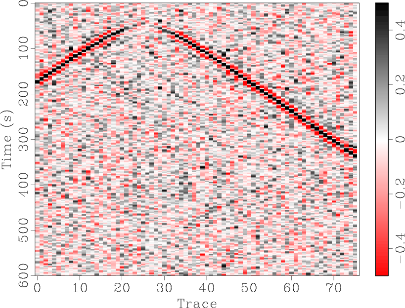
Figure 6. Comparison of denoising effects. (a) Clean data. (b) Gaussian white noise. (c) Noisy data. (d) Denoised result by |
|
|
The third synthetic example is a benchmark data set from SeismicLab. The central frequency of the Ricker wavelet is 40 Hz and the temporal sampling is 2 ms. The number of time samples is 750 and the number of spatial samples is 50. Figures 6(a), 6(b), and 6(c) denote the clean data, noise section, and noisy section, respectively. The SNR in Figure 6(c) is 2.0. Figures 6(d), 6(e), and 6(f) are the denoised results using ![]() predictive filtering,
predictive filtering, ![]() EMD, and
EMD, and ![]() EMDPF, respectively. From removed noise sections Figures 6(g), 6(h), and 6(i) we can conclude that
EMDPF, respectively. From removed noise sections Figures 6(g), 6(h), and 6(i) we can conclude that ![]() predictive filtering harms much useful energy when the number of dip components increases, whereas
predictive filtering harms much useful energy when the number of dip components increases, whereas ![]() EMD affects most of the dipping events, and
EMD affects most of the dipping events, and ![]() EMDPF preserves the useful energy to the greatest extent while removing the slightly weaker level of noise. In this example, the first IMF is removed for prediction in the process of
EMDPF preserves the useful energy to the greatest extent while removing the slightly weaker level of noise. In this example, the first IMF is removed for prediction in the process of ![]() EMDPF.
EMDPF.
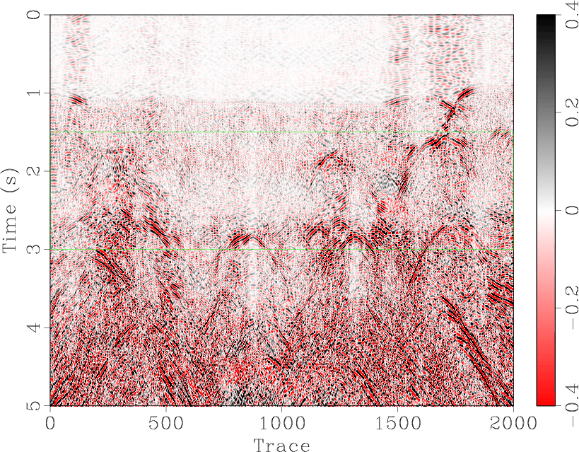
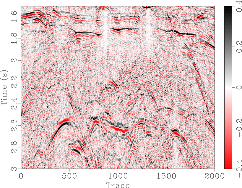
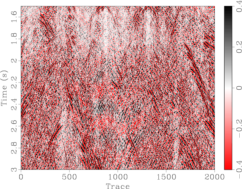
The field data is shown in Figure 7. It is a stacked section without migration from the South China Sea. Figure 7(b) is a zoomed portion of Figure 7(a) from 1.5s to 3.0s. The denoised profiles, shown in Figures 8(a), 8(c), and 8(e), demonstrate ![]() predictive filtering,
predictive filtering, ![]() EMD, and
EMD, and ![]() EMDPF, respectively. The corresponding noise sections are shown in Figures 8(b), 8(d), and 8(f). From these noise sections, we see clearly that
EMDPF, respectively. The corresponding noise sections are shown in Figures 8(b), 8(d), and 8(f). From these noise sections, we see clearly that ![]() EMD removes many dipping events. Even though we can't see clearly the improvement after applying
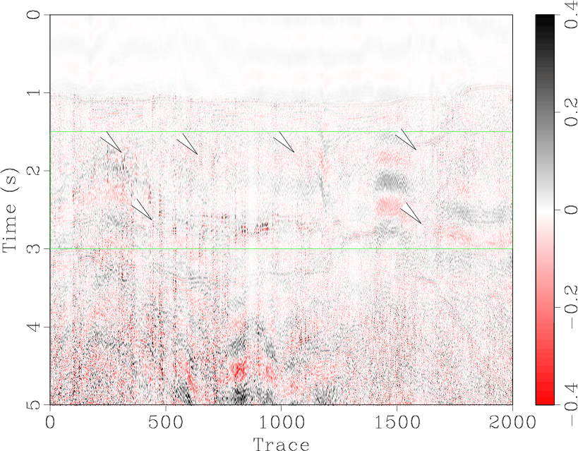
EMD removes many dipping events. Even though we can't see clearly the improvement after applying ![]() EMDPF at the scale of Figure 8, the improvement can be identified on the zoomed noise sections shown in Figure 9. The useful energy shown around 1.75s, 2.6s in Figure 9(b) does not exist in the same part of Figure 9(f). From these differences, we conclude that
EMDPF at the scale of Figure 8, the improvement can be identified on the zoomed noise sections shown in Figure 9. The useful energy shown around 1.75s, 2.6s in Figure 9(b) does not exist in the same part of Figure 9(f). From these differences, we conclude that ![]() EMDPF is more satisfactory than
EMDPF is more satisfactory than ![]() predictive filtering and
predictive filtering and ![]() EMD, in that it leaves less useful energy in the noise section. In this real data example, we apply the AR model on the first three IMFs for
EMD, in that it leaves less useful energy in the noise section. In this real data example, we apply the AR model on the first three IMFs for ![]() EMDPF. For display reasons, the noise sections have been amplified by 3 times.
EMDPF. For display reasons, the noise sections have been amplified by 3 times.


|
|---|
|
southsea,southsea-zoom
Figure 7. Field data from the South China Sea. (a) Original post-stack pre-migration profile. (b) Temporal zoomed part from 1.5s to 3.0s. |
|
|


|
|---|
|
southsea-fxdecon,southsea-fxdecon-noise,southsea-fxemd,southsea-fxemd-noise,southsea-fxemdpf,southsea-fxemdpf-noise
Figure 8. Comparisons between denoised results and corresponding noise sections. (a) Denoised result by |
|
|


|
|---|
|
southsea-fxdecon-zoom,southsea-fxdecon-noise-zoom1,southsea-fxemd-zoom,southsea-fxemd-noise-zoom,southsea-fxemdpf-zoom,southsea-fxemdpf-noise-zoom1
Figure 9. Zoomed part of denoised results and corresponding noise sections. (a) Denoised result by |
|
|
|
|
|
|
Random noise attenuation by |