|
|
|
|
Random noise attenuation by |
Since the frequency of each IMF decreases according to the order in which it is separated out, by subtracting the first few IMFs of each frequency slice in the ![]() domain, we extract the higher wavenumber components, which represent the energy of random noise and high-dip-angle events in seismic sections.
domain, we extract the higher wavenumber components, which represent the energy of random noise and high-dip-angle events in seismic sections.
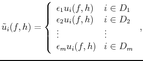
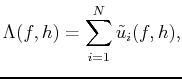
If we divide the set of IMFs into more-detailed zones, we can separate the section into several dip bands. Thus, we reach the definition of the EMD based dip filter:
where
![]() is the filtered data for frequency slice
is the filtered data for frequency slice ![]() in the
in the ![]() domain.
domain.
![]() is the
is the ![]() th separated IMF such that
th separated IMF such that
![]() , where
, where ![]() is the transformed
is the transformed ![]() domain seismic data.
domain seismic data.
![]() is the
is the ![]() th of
th of ![]() , the number of dip bands, and
, the number of dip bands, and
![]() is the corresponding weighting coefficient. For a simple high-pass dip filter, we choose
is the corresponding weighting coefficient. For a simple high-pass dip filter, we choose ![]() ,
,
![]() ,
,
![]() and
and
![]() ,
,
![]() .
.
Figure 3 demonstrates how an EMD based dip filter works on a synthetic plane-wave seismic profile containing three events corresponding to three dips. After filtering with high-pass, mid-pass, and low-pass dip filters, respectively, the three plane waves are successfully separated . The parameters we choose in designing these three filters are shown in Table 1.
| Type | ||||
| high-pass | 10 | 2 |
|
|
| mid-pass | 10 | 3 |
|
|
| low-pass | 10 | 2 |
|
|
The EMD based dip filter is defined adaptively since the filtering process is data driven. We only need to define the number of IMFs contained in each dip band at the start, a step that is convenient to implement.
If we consider random noise as high-dip-angle components, then ![]() EMD denoising (Bekara and van der Baan, 2009) is equivalent to applying a high-cut dip filter with the form of equation 7 to the seismic data in order to remove both random noise and ground roll. We can also understand
EMD denoising (Bekara and van der Baan, 2009) is equivalent to applying a high-cut dip filter with the form of equation 7 to the seismic data in order to remove both random noise and ground roll. We can also understand ![]() EMDPF from EMD based dip filter.
EMDPF from EMD based dip filter. ![]() EMDPF first uses an EMD based dip filter to separate the high-dip-angle and low-dip-angle components, where the high-dip-angle components are composed of steeply dipping useful events and noise, and low-dip-angle components are all useful signals. The useful signal in the high-dip-angle components are predicted and subsequently restored. Due to the effects of the EMD based dip filter, a decrease occurs in the number of useful signal components that needs to be predicted. This decrease results in more accurate overall performance when compared with conventional predictive filtering.
EMDPF first uses an EMD based dip filter to separate the high-dip-angle and low-dip-angle components, where the high-dip-angle components are composed of steeply dipping useful events and noise, and low-dip-angle components are all useful signals. The useful signal in the high-dip-angle components are predicted and subsequently restored. Due to the effects of the EMD based dip filter, a decrease occurs in the number of useful signal components that needs to be predicted. This decrease results in more accurate overall performance when compared with conventional predictive filtering.


|
|---|
|
plane,planeemd1,planeemd2,planeemd3
Figure 3. Demonstration of EMD based dip filter. (a) Original synthetic profile, (b) with high-pass dip filter, (c) with mid-pass dip filter, (d) with low-pass dip filter. |
|
|
|
|
|
|
Random noise attenuation by |