Random noise attenuation by $f$ -$x$ empirical mode decomposition predictive filtering

f-x predictive filtering

Let $s(t,h)(h=1,2,\cdots,H)$ be the signal of trace $h$ and $H$ be the number of traces. If the slope of a linear event with constant amplitude in a seismic section is $\psi$ , then:

$$s(t,h+1)=s(t-h\psi\Delta x,1),$$ (1)

where $\Delta x$ denotes the trace interval. Equation 1 can be transformed into the frequency domain in order to give:

$$S(f,h+1)=S(f,1)e^{-i2\pi fh\psi\Delta x}.$$ (2)

For a specific frequency $f_0$ , from equation 2 we can obtain a linear recursion, which is given by:

$$S(f_0,h+1)=a(f_0,1)S(f_0,h),$$ (3)

where $a(f_0,1)=e^{-i2\pi f_0\psi\Delta x}$ . This recursion is a first-order difference equation, also known as an auto-regressive (AR) model of order 1. Similarly, superposition of $p$ linear events in the $t-x$ domain can be represented by an AR model of order $p$ (Harris and White, 1997; Tufts and Kumaresan, 1980) as the following equation:

$$S(f_0,h+1)=a(f_0,1)S(f_0,h)+a(f_0,2)S(f_0,h-1)+\cdots+a(f_0,p)S(f_0,h+1-p),$$ (4)

where $a(f_0,h)(h=1,2,\cdots,p)$ denotes the predictive error filter, with a length of $p$ . The prediction error energy $E(f_0)$ is given by the following equation:

$$E(f_0)={\Arrowvert a(f_0,h) \ast S(f_0,h)-S(f_0,h+1) \Arrowvert}_2^2,$$ (5)

where symbol $*$ denotes convolution, and $\Arrowvert\cdot\Arrowvert_2^2$ denotes the least-squares energy. By minimizing the prediction error energy $E(f_0)$ , we can get the filtering operator $a(f_0,m)$ . Applying this operator to the spatial trace yields the denoised results for the frequency slice $f_0$ .

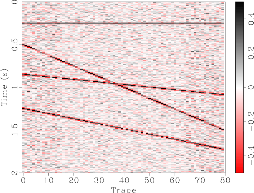
$f-x$ predictive filtering works perfectly on a single event. Figures 1(a)-1(c) show and compare the denoised results for a single flat synthetic event. The denoised result (Figure 1(b)) is quite good, with the random noise in Figure 1(a) largely removed and only a small amount of the useful component in the noise section, Figure 1(c). For a single dipping event, Figures 1(d)-1(f), the results are similar. However, when the number of different dips is increased, the seismic section becomes more complex and predictive filtering is not as effective. Figure 1(j) shows a synthetic section containing four events with differing dips. In the removed noise section, Figure 1(i), there remains a significant amount of residual useful energy.

The synthetic data shown in Figures 1(a), 1(d), and 1(j) were all generated by SeismicLab (Sacchi, 2008), with a signal-to-noise ratio (SNR) of 2.0 for all of them. Here we define the SNR as the ratio of maximum amplitude of useful energy and the maximum amplitude of Gaussian white noise. Note that the same parameters were used for the predictive filters in each case shown in Figure 1.

We now conclude that the effectiveness of $f-x$ predictive filtering deteriorates as the number of different dips increases, mainly because the total of leaked useful energy increases at the same time. In particular, when the number of dips is extremely large, as occurs with hyperbolic events, $f-x$ predictive filtering fails to achieve acceptable results. It is natural to infer that if we can first reduce the number of dips, or in other words pick the very steep events and total random noise out, then by applying the same $f-x$ predictive filtering, the predictive precision will improve. That is the subject of the section on $f-x$ empirical mode decomposition predictive filtering.

syn01-flat,syn01-flat-fxdecon,syn01-flat-fxdecon-noise,syn01-dip,syn01-dip-fxdecon,syn01-dip-fxdecon-noise,syn01-complex,syn01-complex-fxdecon,syn01-complex-fxdecon-noise,syn01-complex,syn01-complex-fxemdpf,syn01-complex-fxemdpf-noise
Figure 1. Demonstration of $f-x$ predictive filtering (a-i) and $f-x$ EMDPF (j-l) on synthetic section with different number of dip components. (a) Single flat event. (b) Denoised single flat event. (c) Removed noise section corresponding to (a) and (b). (d) Single dipping event. (e) Denoised single dipping event. (f) Removed noise section corresponding to (d) and (e). (g) Complex events section. (h) Denoised complex events section. (i) Removed noise section corresponding to (g) and (h). (j) Same as (g). (k) Denoised result by $f-x$ EMDPF. (l) Removed noise section corresponding to (j) and (k).

Random noise attenuation by $f$ -$x$ empirical mode decomposition predictive filtering