Recursive integral time extrapolation of elastic waves using low-rank symbol approximation

Low-rank approximation

So far, we have laid out our basic theory of recursive integral time extrapolation of elastic waves. In mildly heterogeneous media, the Christoffel matrix is SPD. In strongly heterogeneous media, the Christoffel matrix becomes complex-valued and non-Hermitian. However, in both cases, the eigenvalues and eigenvectors of the Christoffel matrix become dependent on both spatial location and propagation direction, in other words, they are functions of both space $\mathbf{x}$ and wavenumber $\mathbf{k}$ . If these operators are implemented straightforwardly, one is faced with the daunting task of computing and storing the complete eigenvalue decomposition of the Christoffel matrix using all the combinations of $\mathbf{x}$ and $\mathbf{k}$ , leading to $\mathcal{O}(N_x^2)$ computational and memory complexity, where $N_x$ refers to the total number of mesh points in $3$ D. To perform wave extrapolation in the form of integral operators, one would have to multiply matrices with vectors in dimension of $N_x$ , leading to a computational complexity of $\mathcal{O}(N_x^2)$ . This is simply infeasible for practical applications.

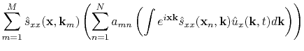
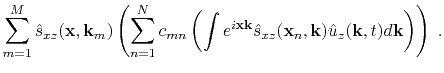
In this work, to efficiently apply the derived Fourier Integral Operators (FIOs), we proposed to apply the low-rank decomposition (Fomel et al., 2013) on the mixed-domain wave extrapolation matrices. Take the wave extrapolation operator in equation 27, $e^{i\Phi \Delta t}$ , as an example. We propose to apply low-rank approximation on each individual element of its expansion. For instance, the $\hat{s}_{xx}$ element, which operates on the x-component of the input vector wavefield and outputs to the x-component of the output vector wavefield, can be approximated as (Fomel et al., 2013):

$$\hat{s}_{xx}(\mathbf{x},\mathbf{k}) \approx \sum\limits_{m=1}^M \... ...}_{xx}(\mathbf{x},\mathbf{k}_m) a_{mn} \hat{s}_{xx}(\mathbf{x}_n,\mathbf{k})\;,$$ (29)

where $\hat{s}_{xx}(\mathbf{x},\mathbf{k}_m)=\mathbf{U}$ and $\hat{s}_{xx}(\mathbf{x}_n,\mathbf{k})=\mathbf{V}^*$ are sampled representative columns and rows from the original matrix $\hat{s}_{xx}(\mathbf{x},\mathbf{k})=\mathbf{W}$ , $M$ and $N$ are the numerical ranks of matrix $\mathbf{W}$ , and the matrix $a_{mn}=\mathbf{A}$ is obtained from minimizing

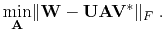$$\min_{\mathbf{A}} \lVert \mathbf{\mathbf{W} - \mathbf{U} \mathbf{A} \mathbf{V}^*} \rVert_F \;.$$ (30)

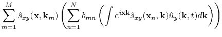
Similarly, $\hat{s}_{xy}$ and $\hat{s}_{xz}$ can be approximated as:

$$\hat{s}_{xy}(\mathbf{x},\mathbf{k}) \approx \sum\limits_{m=1}^M \sum\limits_{n=1}^N \hat{s}_{xy}(\mathbf{x},\mathbf{k}_m) b_{mn} \hat{s}_{xy}(\mathbf{x}_n,\mathbf{k})\;,$$ (31)

$$\hat{s}_{xz}(\mathbf{x},\mathbf{k}) \approx \sum\limits_{m=1}^M \sum\limits_{n=1}^N \hat{s}_{xz}(\mathbf{x},\mathbf{k}_m) c_{mn} \hat{s}_{xz}(\mathbf{x}_n,\mathbf{k})\;.$$ (32)

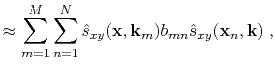
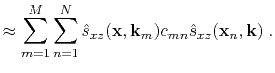
The computation of $\hat{u}_x(\mathbf{x},t+\Delta t)$ then becomes:

$$\hat{u}_x(\mathbf{x},t+\Delta t) \approx \sum\limits_{m=1}^M \hat{s}_{xx}(\mathbf{x},\mathbf{k}_m) \left( ... ...x}(\mathbf{x}_n,\mathbf{k}) \hat{u}_x(\mathbf{k},t) d\mathbf{k} \right) \right)$$ (33)

$$+ \sum\limits_{m=1}^M \hat{s}_{xy}(\mathbf{x},\mathbf{k}_m) \left( ... ...y}(\mathbf{x}_n,\mathbf{k}) \hat{u}_y(\mathbf{k},t) d\mathbf{k} \right) \right)$$

$$+ \sum\limits_{m=1}^M \hat{s}_{xz}(\mathbf{x},\mathbf{k}_m) \left( ... ...mathbf{x}_n,\mathbf{k}) \hat{u}_z(\mathbf{k},t) d\mathbf{k} \right) \right) \;.$$

The computation of $y$ and $z$ components can be carried out in a similar fashion. The computational cost of applying each FIO reduces to a complexity of $\mathcal{O}(N N_x \log N_x)$ , where $\mathcal{O}(N_x \log N_x)$ is the complexity of one forward or inverse Fast Fourier Transform (FFT), and $N$ is the numerical rank of the low-rank approximation, which is $1$ for homogeneous media and $\mathcal{O}(1)$ for heterogeneous media.

Recursive integral time extrapolation of elastic waves using low-rank symbol approximation