|
 |
 |
 | Recursive integral time extrapolation of elastic waves using low-rank symbol approximation |  |
![[pdf]](icons/pdf.png) |
Next: Low-rank approximation
Up: Theory
Previous: Homogeneous Media
In heterogeneous media, the elastic wave equation can be expressed using the Einstein notation:
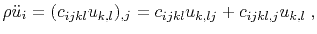 |
(23) |
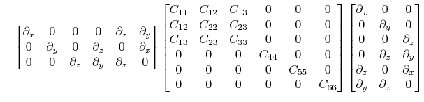
where dot on top denotes time derivative, comma in subscript denotes spatial derivative and repeated indices imply summation. Analogously, the Christoffel matrix  in the case of orthorhombic symmetry can be expanded using the chain rule
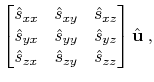
After spatial Fourier transform,
 . The Christoffel matrix
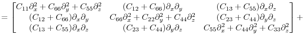
 in the case of orthorhombic anisotropy takes the form:
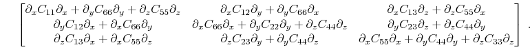
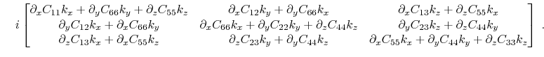
When the model is smoothly varying, which is the underlying assumption of wave mode separation (Cheng et al., 2014), the gradients of stiffnesses are insignificant. In such cases, the imaginary matrix can be dropped, which leads to the conventional real-valued Christoffel matrix in Equation 12. However, in the case of strong heterogeneity, such as at medium interfaces, the gradients of stiffnesses become significant and the imaginary part needs to be taken into account. Because
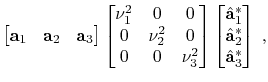
becomes complex and non-Hermitian, the eigendecomposition of the generic matrix
 is expressed as
where the superscript  denotes conjugate transpose. Note that the eigenvalues
 and
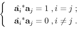
and  , as well as their corresponding eigenvectors, are complex-valued. Since
 is square and
 :
:
Physically, this means in strongly heterogeneous media, wave mode separation cannot be clearly defined due to wave mode conversion, which is expressed as the imaginary part of eigenvalues. The polarization directions are no longer orthogonal in the real sense - they become orthogonal complex vectors.
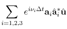
The situation stated above does not prevent our framework from performing the correct wavefield extrapolation. The wave extrapolation operator then becomes
where
Comparing equation 27 with equation 16, we can see that because the eigenvalues that appear in the exponent in equation 27 are no longer real-valued, the corresponding two-step operators to that in equation 20 cannot be constructed using Euler's formula.
|
|
|
|
| Recursive integral time extrapolation of elastic waves using low-rank symbol approximation | |
|
Next: Low-rank approximation
Up: Theory
Previous: Homogeneous Media
2018-11-16