|
|
|
|
Effects of lateral heterogeneity on time-domain processing parameters |
Next: Appendix B Derivation of Up: Appendix A Review of Previous: Reflection traveltime
|
|
|
|
Effects of lateral heterogeneity on time-domain processing parameters |
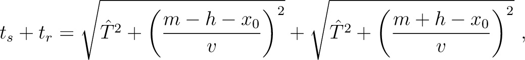
As a more fundamental alternative to study seismic responses, one can choose to consider a reflecting point (scatterer) instead of a reflecting surface because any model is a superposition of such scatterers. Assuming that the subsurface velocity  is constant, the total (diffraction) traveltime of the wave traveling in this configuration is simply a sum of traveltime of the two legs, which can be expressed by the double-square-root (DSR) equation (Claerbout, 1996):
 denotes midpoint,
  denotes half offset,
  denotes the horizontal coordinate of the point scatterer, and
  is a one-way vertical traveltime from the point scatterer to the surface. The true location of the point scatterer will also be the same as the emerging location of the image rays (Hubral, 1977).
In the more general case of varying subsurface velocity, equation (32) becomes an approximation for diffraction traveltime that is routinely used in prestack time migration (Yilmaz, 2001). then denotes the one-way traveltime of the image ray from the point scatter to the surface and the escape location of the image ray will generally be different from the true location of the point scatterer in the Cartesian coordinates. The velocity becomes time-migration velocity  , which will be selected for the best fit traveltime to equation (32).
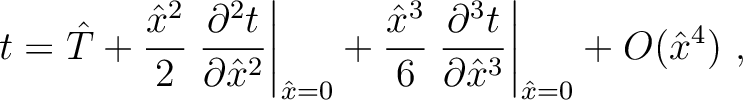
To further understand equation (32) in heterogeneous media, we follow the derivation by () and consider the general one-way traveltime approximation centered around the image ray from the point scatterer to any surface point  given by,
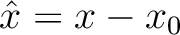 denotes the distance between the escape location and any surrounding point on the surface. Note that
  functions similarly to in equation (5) but has a different meaning than the conventional half offset when considering reflection traveltime. The first-order term in equation (33) is always equal to zero due to the image rays always having zero phase slowness tangent to the surface, or equivalently to
 at
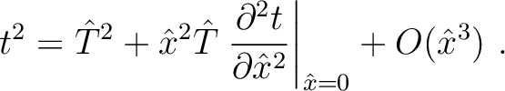
at  . We emphasize the notable presence of possible third-order term (
 ). This term can be neglected when is sufficiently small or when the medium under consideration provides additional symmetry to the function of traveltime such as in homogeneous or horizontally layered VTI media, where traveltime varies as an even function around . Converting equation (33) to a series in traveltime squared gives
Using equation (34), we can compute the total traveltime from a source at
). This term can be neglected when is sufficiently small or when the medium under consideration provides additional symmetry to the function of traveltime such as in homogeneous or horizontally layered VTI media, where traveltime varies as an even function around . Converting equation (33) to a series in traveltime squared gives
Using equation (34), we can compute the total traveltime from a source at  to point scatterer and to a receiver at
  as follows,
Equation (35) suggests that equation (32) simply represents a sum of two Taylor expansions of the one-way traveltime from the point scatterer to the source and the receiver. Therefore, the migration velocity can be related to the one-way traveltime derivatives as shown in equation (7). Moreover, our proposed framework to study the effects of weak lateral heterogeneity on one-way traveltime is applicable to
as follows,
Equation (35) suggests that equation (32) simply represents a sum of two Taylor expansions of the one-way traveltime from the point scatterer to the source and the receiver. Therefore, the migration velocity can be related to the one-way traveltime derivatives as shown in equation (7). Moreover, our proposed framework to study the effects of weak lateral heterogeneity on one-way traveltime is applicable to  provided that the image ray is assumed to be sufficiently close to the vertical direction, which is exactly true in the case of 1D layered anisotropic media with horizontal symmetry planes.
|
|
|
|
Effects of lateral heterogeneity on time-domain processing parameters |