 |
 |
 |
 | Velocity continuation by spectral methods |  |
![[pdf]](icons/pdf.png) |
Next: Conclusions
Up: Fomel: Spectral velocity continuation
Previous: Suppressing wraparound artifacts of
For an alternative spectral approach, I adopted the Chebyshev- method (Lanczos, 1956; Gottlieb and Orszag, 1977). The Chebyshev- velocity continuation
algorithm consists of the following steps:
method (Lanczos, 1956; Gottlieb and Orszag, 1977). The Chebyshev- velocity continuation
algorithm consists of the following steps:
- Transform the regular grid in
 to Gauss-Lobato collocation
points, required for the fast Chebyshev transform. First, a new
variable
to Gauss-Lobato collocation
points, required for the fast Chebyshev transform. First, a new
variable  is introduced by the shift transform:
 |
(10) |
so that the domain
 is mapped into the domain
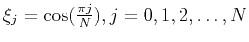
 . Second, the grid points are distributed
regularly in the cosine projection:
. Second, the grid points are distributed
regularly in the cosine projection:
 .
.
- Transform the initial image
 into the Chebyshev space
in and Fourier transform in
into the Chebyshev space
in and Fourier transform in  , using the FFT algorithm. The
Chebyshev-Fourier representation of is
, using the FFT algorithm. The
Chebyshev-Fourier representation of is
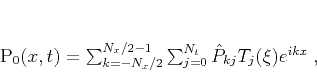 |
(11) |
where  denotes the Chebyshev polynomial of degree
  .
.
- Apply equation (1) to advance the image in velocity
 .
It is convenient to rewrite this equation in the form
.
It is convenient to rewrite this equation in the form
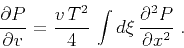 |
(12) |
In the Chebyshev- domain, the double differentiation in is
performed by multiplying the Fourier transform of  by
by  , and
integration in is performed
as a direct operations on the Chebyshev coefficients. In
particular, if
, and
integration in is performed
as a direct operations on the Chebyshev coefficients. In
particular, if
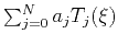 is the Chebyshev
representation of the function
is the Chebyshev
representation of the function  , then the coefficients
 of
of
 are defined by the relation
 |
(13) |
where  ,
,  for
for  , and
, and  for
for  .
The constant of integration (and, correspondingly, the coefficient
.
The constant of integration (and, correspondingly, the coefficient
 ) can be found at each velocity step from the boundary
conditions (2), which are transformed to the form
) can be found at each velocity step from the boundary
conditions (2), which are transformed to the form
 |
(14) |
For the velocity advancement I used an implicit Crank-Nicolson scheme,
which is unconditionally stable independent of the velocity step size.
By writing equation (12) in the matrix form
 |
(15) |
the Crank-Nicolson advancement is represented by the equation
 |
(16) |
where  is the identity matrix. The inverted matrix
 has a tridiagonal
structure, except for the first row, implied by the boundary
condition (14). A careful treatment of the boundary
condition by the matrix-bordering method (Boyd, 1989; Faddeev and Faddeeva, 1963) allows
for an efficient inversion at a tridiagonal solver speed.
has a tridiagonal
structure, except for the first row, implied by the boundary
condition (14). A careful treatment of the boundary
condition by the matrix-bordering method (Boyd, 1989; Faddeev and Faddeeva, 1963) allows
for an efficient inversion at a tridiagonal solver speed.
- Transform the result of the velocity advancement back to the
physical domain.
- Transform the grid back to being regularly space in .
|
|---|
cheb1
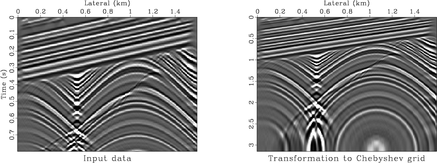
Figure 6. Synthetic seismic data before (left) and
after (right) transformation to the Chebyshev grid in squared time.
|
|---|
![[png]](icons/viewmag.png) ![[scons]](icons/configure.png)
|
|---|
|
|---|
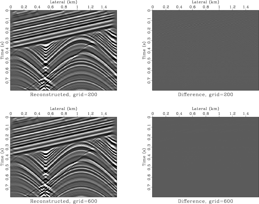
cheb1-inv
Figure 7. The left plots show the reconstruction of the original data
after transforming back from the Chebyshev grid to the original
grid. The right plots show the difference with the original model.
Top: using the original grid size ( ). Bottom: increasing
the grid size by a factor of three. ). Bottom: increasing
the grid size by a factor of three.
|
|---|
|
|
|---|
The first advantage of the Chebyshev approach comes from the better
conditioning of the grid transform. Figure 6 shows the
synthetic data before and after the grid transform. Figure
7 shows a reconstruction of the original data after
transforming back from the Chebyshev grid (Gauss-Lobato collocation
points). The difference with the original image is negligibly small.
|
|---|
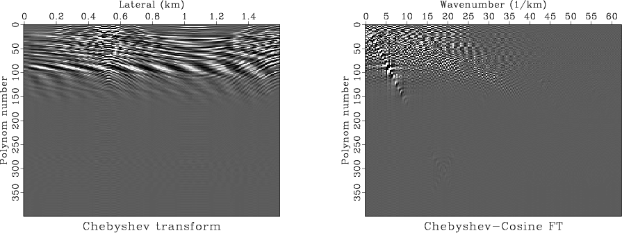
cheb1-fft
Figure 8. Left: Synthetic data after Chebyshev
transform. Right: the real part of the Fourier transform in the
space coordinate.
|
|---|
|
|
|---|
The second advantage is the compactness of the Chebyshev
representation. Figure 8 shows the data after the
decomposition into Chebyshev polynomials in and Fourier
transform in . We observe a very rapid convergence of the Chebyshev
representation: a relatively small number of polynomials suffices to
represent the data.
|
|---|
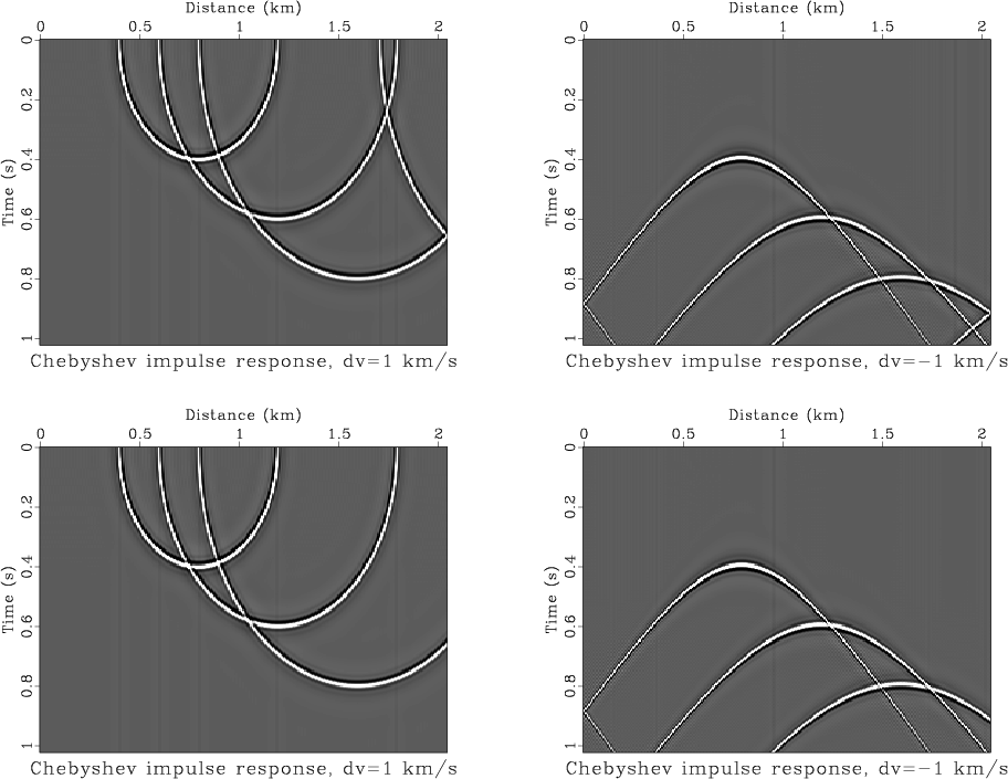
cheb-impl
Figure 9. Impulse responses (Green's functions) of
velocity continuation, computed by the Chebyshev- method. Top:
without zero padding, bottom: with zero padding on the axis. The
left plots correspond to continuation to a larger velocity ( km/sec); the right plots, smaller velocity, (
 km/sec). km/sec).
|
|---|
|
|
|---|
The third advantage is the proper handling of the non-periodic boundary
conditions. Figure 9 shows the velocity continuation
impulse responses, computed by the Chebyshev method. As expected, no
wraparound artifacts occur on the time axis, and the accuracy of the
result is noticeably higher than in the case of finite differences
(Figure 1).
|
|
|
|
| Velocity continuation by spectral methods | |
|
Next: Conclusions
Up: Fomel: Spectral velocity continuation
Previous: Suppressing wraparound artifacts of
2013-03-03