Forward interpolation

Function basis

A particular form of the solution (1) arises from assuming the existence of a basis function set $\{\psi_k(x)\},\;k \in K$, such that the function $f (x)$ can be represented by a linear combination of the basis functions in the set, as follows:

$$f (x) = \sum_{k \in K} c_k \psi_k (x)\;.$$ (8)

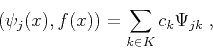
We can find the linear coefficients $c_k$ by multiplying both sides of equation (8) by one of the basis functions (e.g. $\psi_j (x)$). Inverting the equality

$$\left( \psi_j (x), f (x)\right) = \sum_{k \in K} c_k \Psi_{jk}\;,$$ (9)

where the parentheses denote the dot product, and

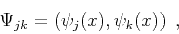$$\Psi_{jk} = \left( \psi_j (x), \psi_k (x)\right) \;,$$ (10)

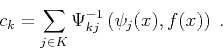
leads to the following explicit expression for the coefficients $c_k$:

$$c_k = \sum_{j \in K} \Psi^{-1}_{kj} \left( \psi_j (x), f (x)\right) \;.$$ (11)

Here $\Psi^{-1}_{kj}$ refers to the $kj$ component of the matrix, which is the inverse of $\Psi$. The matrix $\Psi$ is invertible as long as the basis set of functions is linearly independent. In the special case of an orthonormal basis, $\Psi$ reduces to the identity matrix:

$$\Psi_{jk} = \Psi^{-1}_{kj} = \delta_{jk}\;.$$ (12)

Equation (11) is a least-squares estimate of the coefficients $c_k$: one can alternatively derive it by minimizing the least-squares norm of the difference between $f (x)$ and the linear decomposition (8). For a given set of basis functions, equation (11) approximates the function $f (x)$ in formula (1) in the least-squares sense.

Forward interpolation