|
|
|
|
Exploring three-dimensional implicit wavefield extrapolation with the helix transform |
|
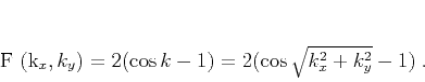
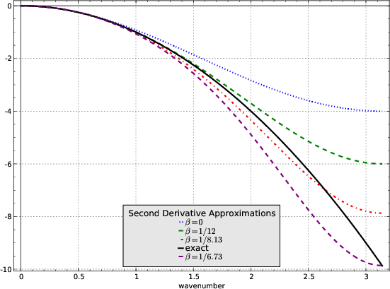
sixth Figure A-1. The second-derivative operator in the wavenumber domain and its approximations. |
|
|---|---|
|
|
|
|---|
|
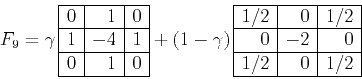
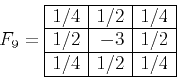
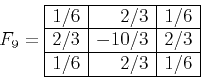
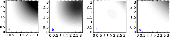
laplace Figure B-1. The numerical anisotropy error of different Laplacian approximations. Both the five-point Laplacian (plot a) and its rotated version (plot b) are accurate along the axes, but exhibit significant anisotropy in between at large wavenumbers. The nine-point McClellan filter (plot c) has a reduced error, while the filter with |
|
|
Under the helix transform, a filter of the general form
(B-2) becomes equivalent to a one-dimensional filter with
the ![]() transform
transform
|
|---|
|
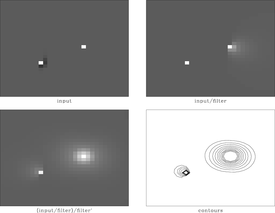
inv-laplace Figure B-2. Inverting the Laplacian operator by a helix deconvolution. The top left plot shows the input, which contains a single spike and the causal minimum-phase filter |
|
|
|
|
|
|
Exploring three-dimensional implicit wavefield extrapolation with the helix transform |
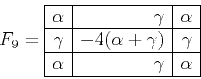
![\begin{displaymath}
F_9 (k_x,k_y) = 4\,\alpha\,[\cos{k_x}\,\cos{k_y} - 1] +
2\,\gamma\,[\cos{k_x}+\cos{k_y}-2]\;,
\end{displaymath}](img95.png)