 |
 |
 |
 | Exploring three-dimensional implicit wavefield extrapolation
with the helix transform |  |
![[pdf]](icons/pdf.png) |
Next: Spectral factorization and three-dimensional
Up: Fomel & Claerbout: Implicit
Previous: Introduction
The difference between implicit and explicit extrapolation is best
understood through an example. Following Claerbout (1985),
let us consider, for instance, the diffusion (heat conduction) equation
of the form
 |
(1) |
Here  denotes time,
  is the space coordinate,
  is the
temperature, and
is the
temperature, and  is the heat conductivity coefficient.
Equation (1) forms a well-posed boundary-value problem if
supplied with the initial condition
is the heat conductivity coefficient.
Equation (1) forms a well-posed boundary-value problem if
supplied with the initial condition
 |
(2) |
and the appropriate boundary conditions. Our task is to build a
digital filter, which transforms a gridded temperature  from one
time level to another.
from one
time level to another.
It helps to note that when the conductivity coefficient is
constant and the space domain of the problem is infinite (or periodic)
in , the problem can be solved in the wavenumber domain. Indeed,
after the Fourier transform over the variable , equation
(1) transforms to the ordinary differential equation
 |
(3) |
which has the explicit analytical solution
 |
(4) |
where  denotes the Fourier transform of , and
  stands
for the wavenumber. Therefore, the desired filter in the
wavenumber domain has the form
stands
for the wavenumber. Therefore, the desired filter in the
wavenumber domain has the form
 |
(5) |
where for simplicity the coefficient is normalized for the time
step  equal to
  .
.
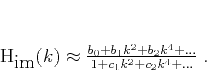
Returning now to the time-and-space domain, we can approach the filter
construction problem by approximating the space-domain response of
filter (5) in terms of the differential operators
 , which can be approximated
by finite differences. An explicit approach would amount to
constructing a series expansion of the form
, which can be approximated
by finite differences. An explicit approach would amount to
constructing a series expansion of the form
 |
(6) |
and selecting the coefficients  to approximate equation
(5). For example, the three-term Taylor series expansion
around the zero wavenumber yields
to approximate equation
(5). For example, the three-term Taylor series expansion
around the zero wavenumber yields
 |
(7) |
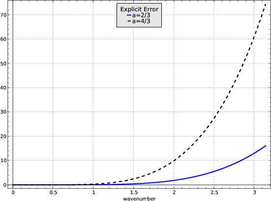
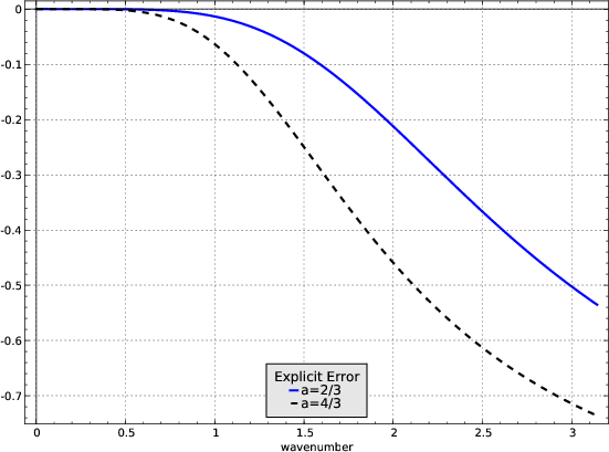
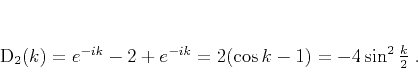
The error of approximation (7) as a function of
for two different values of is shown in the left plot of Figure
1.
|
|---|
exerror,imerror
Figure 1. Errors of second-order
explicit (a) and implicit (b) approximations for the heat extrapolation.
|
|---|
![[png]](icons/viewmag.png) ![[sage]](icons/sage.png)
|
|---|
An implicit approach also approximates the ideal filter
(5), but with a rational approximation of the form
 |
(8) |
One way of selecting the coefficients  and
and  is to apply an
appropriate Padé approximation (Baker and Graves-Morris, 1981)
is to apply an
appropriate Padé approximation (Baker and Graves-Morris, 1981)![[*]](icons/footnote.png) . For example the
. For example the ![$[2/2]$](img26.png) Padé
approximation is
Padé
approximation is
 |
(9) |
This approximation corresponds to the famous Crank-Nicolson implicit
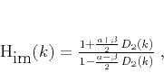
method (Crank and Nicolson, 1947). The error of approximation (9) as
a function of for different values of is shown in the right
plot of Figure 1. Not only is it significantly smaller
than the error of the same-order explicit approximation, but it also
has a negative sign. It means that the high-frequency numerical noise
gets suppressed rather than amplified. In practice, this property
translates into a stable numerical extrapolation.
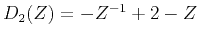
The second derivative operator  can be approximated in practice
by a digital filter. The most commonly used filter has the
can be approximated in practice
by a digital filter. The most commonly used filter has the
 -transform
 , and the Fourier transform
 |
(10) |
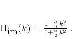
Formula (10) approximates well only for small
wavenumbers . As shown in Appendix A, the implicit scheme allows
the accuracy of the second-derivative filter to be significantly
improved by a variation of the ``1/6-th trick''
(Claerbout, 1985). The final form of the implicit
extrapolation filter is
 |
(11) |
where  is a numerical constant, found in Appendix A.
|
|---|
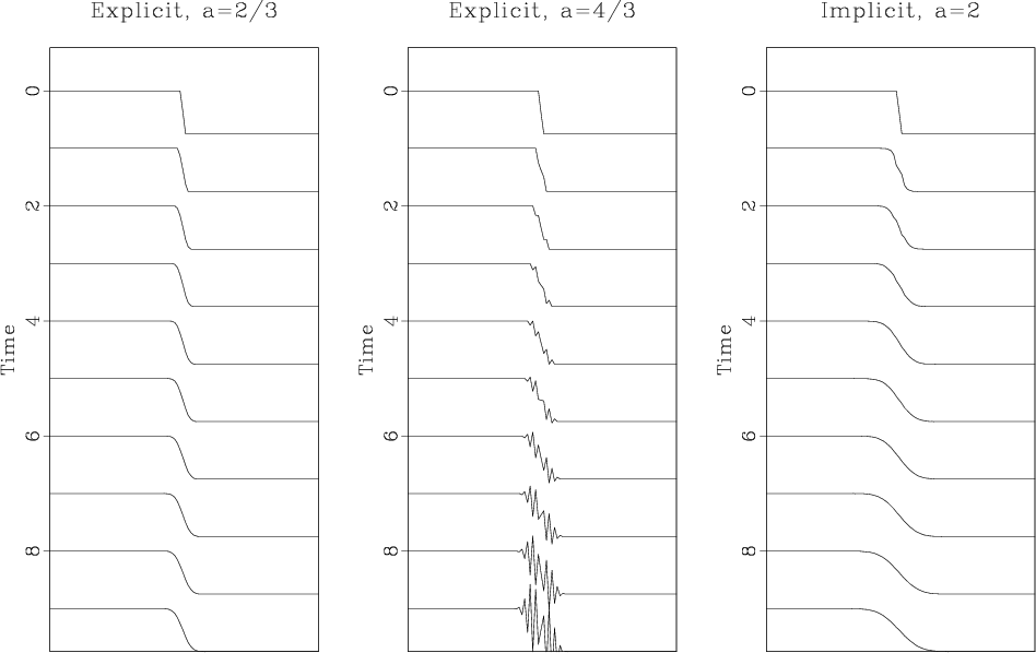
heat
Figure 2. Heat extrapolation with explicit
and implicit finite-different schemes. Explicit extrapolation
appears stable for  (left plot) and unstable for (left plot) and unstable for  (middle plot). Implicit interpolation is stable even for larger
values of (right plot).
(middle plot). Implicit interpolation is stable even for larger
values of (right plot).
|
|---|
![[scons]](icons/configure.png)
|
|---|
A numerical 1-D example is shown in Figure 2. The initial
temperature distribution is given by a step function. The
discontinuity at the step gets smoothed with time by the heat
diffusion. The left plot shows the result of an explicit extrapolation
with , which appears stable. The middle plot is an explicit
extrapolation with , which shows a terribly unstable behavior:
the high-frequency numerical noise is amplified and dominates the
solution. The right plot shows a stable (though not perfectly
accurate) extrapolation with the implicit scheme for the larger value of
 .
.
The difference in stability between explicit and implicit schemes is
even more pronounced in the case of wave extrapolation. For
example, let us consider the ideal depth extrapolation filter in the
form of the phase-shift operator
(Claerbout, 1985; Gazdag, 1978)
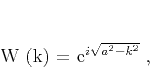 |
(12) |
where
 ,
,  is the time frequency, and
  is the
seismic velocity (which may vary spatially); we assume for simplicity
that both the depth step
is the
seismic velocity (which may vary spatially); we assume for simplicity
that both the depth step  and the space sampling
 are normalized to . A simple implicit approximation
to filter (12) is
are normalized to . A simple implicit approximation
to filter (12) is
 |
(13) |
where
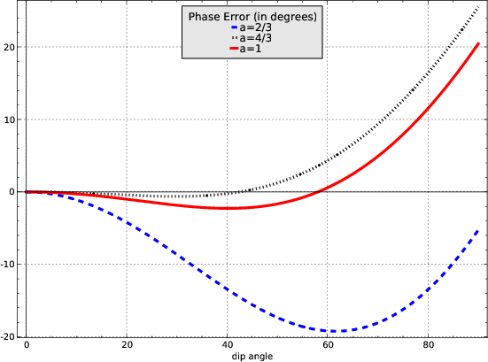
 . We can see
that approximation (13) is again a pure phase shift
operator, only with a slightly different phase. For that reason, the
operator is unconditionally stable for all values of : the total
wave energy from one depth level to another is preserved. Operator
(12) corresponds to the Crank-Nicolson scheme for the
45-degree one-way wave equation (Claerbout, 1985). Its
phase error as a function of the dip angle
. We can see
that approximation (13) is again a pure phase shift
operator, only with a slightly different phase. For that reason, the
operator is unconditionally stable for all values of : the total
wave energy from one depth level to another is preserved. Operator
(12) corresponds to the Crank-Nicolson scheme for the
45-degree one-way wave equation (Claerbout, 1985). Its
phase error as a function of the dip angle
 for different values of is shown in Figure
3.
for different values of is shown in Figure
3.
phase
Figure 3. The phase error of the
implicit depth extrapolation with the Crank-Nicolson method.
|
|
|
|
|---|
The unconditional stability property is not achievable with the
explicit approach, though it is possible to increase the stability of
explicit operators by using relatively long filters
(Hale, 1991b; Holberg, 1988).
|
|
|
|
| Exploring three-dimensional implicit wavefield extrapolation
with the helix transform | |
|
Next: Spectral factorization and three-dimensional
Up: Fomel & Claerbout: Implicit
Previous: Introduction
2014-02-17