|
|
|
|
Kirchhoff migration using eikonal-based computation of traveltime source-derivatives |
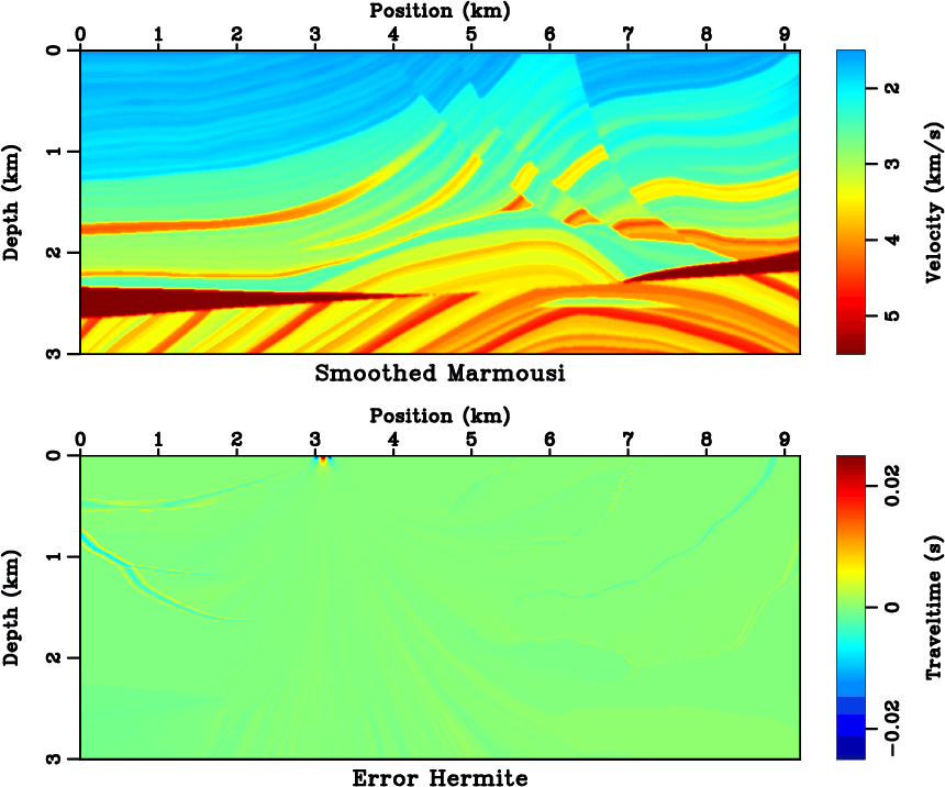
The Marmousi model (Versteeg, 1994) has large velocity variations and is challenging for Kirchhoff
migration with first-arrivals (Geoltrain and Brac, 1993). We apply a single-fold 2D triangular smoothing of
radius ![]() m to the original model (see Figure 9) to remove only sharp velocity discontinuities
but retain the complex velocity structures. Because wave-fronts change shapes rapidly, the traveltime
interpolation may be subject to inaccurate source-derivatives and provide less satisfying accuracy
compared to that in a simple model. Although the derivative computation in the proposed eikonal-based
method is source-sampling independent, in practice we should limit the interpolation interval to be
sufficiently small, so that the traveltime curve could be well represented by a cubic spline. For the
smoothed Marmousi model, we use a sparse source sampling of
m to the original model (see Figure 9) to remove only sharp velocity discontinuities
but retain the complex velocity structures. Because wave-fronts change shapes rapidly, the traveltime
interpolation may be subject to inaccurate source-derivatives and provide less satisfying accuracy
compared to that in a simple model. Although the derivative computation in the proposed eikonal-based
method is source-sampling independent, in practice we should limit the interpolation interval to be
sufficiently small, so that the traveltime curve could be well represented by a cubic spline. For the
smoothed Marmousi model, we use a sparse source sampling of ![]() km based on observations of the
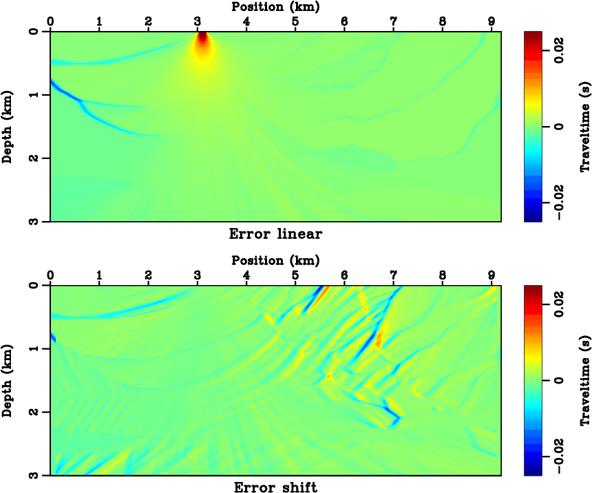
horizontal width of major velocity structures. Figures 9 and 10 compare the
traveltime interpolation errors of three methods as in Figure 3 for a source located
at
km based on observations of the
horizontal width of major velocity structures. Figures 9 and 10 compare the
traveltime interpolation errors of three methods as in Figure 3 for a source located
at ![]() km from nearby source samples at
km from nearby source samples at ![]() km and
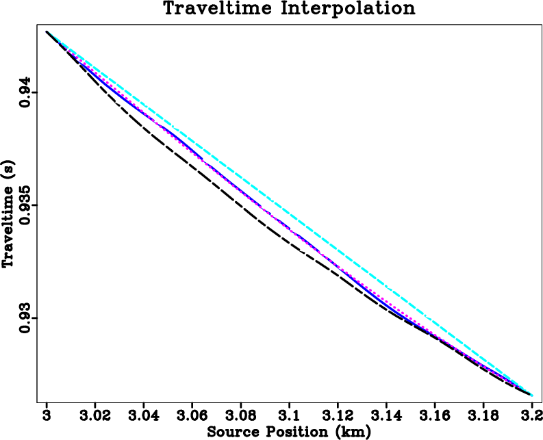
km and ![]() km. Figure 11 plots
a reference traveltime curve for the fixed subsurface location
km. Figure 11 plots
a reference traveltime curve for the fixed subsurface location ![]() km computed by a dense eikonal
solving of
km computed by a dense eikonal
solving of ![]() m source spacing against curves produced by the interpolations. While these comparisons
vary between different source intervals and subsurface locations, the cubic Hermite interpolation
out-performs the linear and the shift interpolations except for the source singularity region. However
in Figure 9 the errors are relatively large in the upper-left region. These errors occur
due to the collapse of overlapping branches of the traveltime field (Xu et al., 2001) that causes wave-front
discontinuities and undermines the assumptions of the proposed method.
m source spacing against curves produced by the interpolations. While these comparisons
vary between different source intervals and subsurface locations, the cubic Hermite interpolation
out-performs the linear and the shift interpolations except for the source singularity region. However
in Figure 9 the errors are relatively large in the upper-left region. These errors occur
due to the collapse of overlapping branches of the traveltime field (Xu et al., 2001) that causes wave-front
discontinuities and undermines the assumptions of the proposed method.
|
|---|
|
vel
Figure 9. (Top) the smoothed Marmousi model. The model has a |
|
|
|
|---|
|
slice
Figure 10. The traveltime error by (top) the linear interpolation and (bottom) the shift interpolation. |
|
|
|
|---|
|
curve
Figure 11. Traveltime interpolation for a fixed subsurface location. Compare between the result from a dense source sampling (solid blue), cubic Hermite interpolation (dotted magenta), linear interpolation (dashed cyan) and shift interpolation (dashed black). The |
|
|
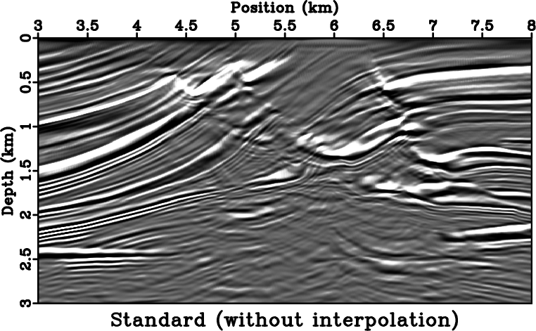
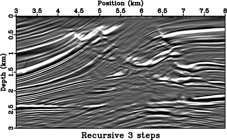
One strategy for imaging multi-arrival wavefields with first-arrival traveltimes is the semi-recursive
Kirchhoff migration (Bevc, 1997). It breaks the image into several depth intervals, applies Kirchhoff
redatuming to the next interval, performs Kirchhoff migration from there, and so on. The small redatuming
depth effectively limits the maximum traveltime and the evolving of complex waveforms before the most
energetic arrivals separate from first-arrivals. Since Kirchhoff redatuming also relies on traveltimes
between datum levels, our method can be fully incorporated into the whole process. Again, for simplicity,
we do not consider amplitude factors during migration. We use the Marmousi dataset with a source/receiver
sampling of ![]() m. Due to the source and receiver reciprocity, the receiver side interpolations are
equivalent to those on the source side. Figure 12 is the result of a Kirchhoff migration
with eikonal solvings at each source/receiver location, i.e. no interpolation performed. Only the upper
portion is well imaged. Figure 13 shows the image after employing the cubic Hermite
interpolation with a
m. Due to the source and receiver reciprocity, the receiver side interpolations are
equivalent to those on the source side. Figure 12 is the result of a Kirchhoff migration
with eikonal solvings at each source/receiver location, i.e. no interpolation performed. Only the upper
portion is well imaged. Figure 13 shows the image after employing the cubic Hermite
interpolation with a ![]() km sparse source/receiver sampling, which means
km sparse source/receiver sampling, which means ![]() source interpolations
within each interval. Even though a
source interpolations
within each interval. Even though a ![]() times speed-up is not attainable in practice due to the extra
computations in source-derivative and interpolation, we are still able to gain an approximately
times speed-up is not attainable in practice due to the extra
computations in source-derivative and interpolation, we are still able to gain an approximately ![]() -fold
cost reduction in traveltime computations, while keeping the image quality comparable between
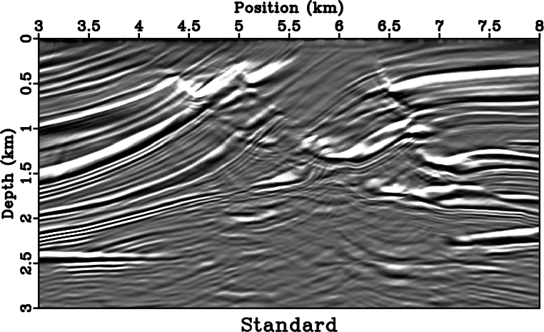
Figures 12 and 13. Next, following Bevc (1997), we downward continue the data
to a depth of
-fold
cost reduction in traveltime computations, while keeping the image quality comparable between
Figures 12 and 13. Next, following Bevc (1997), we downward continue the data
to a depth of ![]() km in three datuming steps. The downward continued data are then Kirchhoff migrated
and combined with the upper portion of Figure 13. We keep the same
km in three datuming steps. The downward continued data are then Kirchhoff migrated
and combined with the upper portion of Figure 13. We keep the same ![]() km sparse
source/receiver sampling whenever eikonal solvings are required in this process. Figure 14
shows the image obtained by the semi-recursive Kirchhoff migration. The target zone at approximately
km sparse
source/receiver sampling whenever eikonal solvings are required in this process. Figure 14
shows the image obtained by the semi-recursive Kirchhoff migration. The target zone at approximately
![]() km appears better imaged.
km appears better imaged.
|
|---|
|
dmig0d
Figure 12. Image of Kirchhoff migration with first-arrivals (no interpolation). |
|
|
|
|---|
|
dmig0
Figure 13. Image of Kirchhoff migration with first-arrivals and a sparse source/receiver sampling. |
|
|
|
|---|
|
dmig2
Figure 14. Image of semi-recursive Kirchhoff migration with a three-step redatuming from top surface to |
|
|
|
|
|
|
Kirchhoff migration using eikonal-based computation of traveltime source-derivatives |