|
|
|
|
Kirchhoff migration using eikonal-based computation of traveltime source-derivatives |
In a 2D medium of linearly changing velocities,
![]() where x is the
lateral position and z is the depth, the traveltimes and source-derivatives have analytical
solutions (Slotnick, 1959). Figure 1 shows the model used in our numerical test
and the analytical source-derivative for a source located at
where x is the
lateral position and z is the depth, the traveltimes and source-derivatives have analytical
solutions (Slotnick, 1959). Figure 1 shows the model used in our numerical test
and the analytical source-derivative for a source located at ![]() km. The domain is of
size 4km
km. The domain is of
size 4km ![]() 4km with grid spacing
4km with grid spacing ![]() km in both directions. We solve for the traveltime
tables at five sources of uniform spacing
km in both directions. We solve for the traveltime
tables at five sources of uniform spacing ![]() km along the top domain boundary by FMM and
their associated source-derivatives using the method described in Appendix A. Figure 2
compares the errors in computed source-derivative between the proposed approach and a centered
second-order finite-difference estimation for the same source shown in Figure 1.
The proposed method is sufficiently accurate except for the small region around the source. This
is due to the source singularity of the eikonal equation and can be improved by adaptive or
high-order upwind finite-difference methods (Qian and Symes, 2002) or by factoring the singularity
(Fomel et al., 2009). Since we are aiming at using the interpolated traveltime tables for migration
purposes and the reflection energy around the sources is usually low, these errors in current
implementation can be neglected. In Figure 3, we interpolate the traveltime
table for a source at location
km along the top domain boundary by FMM and
their associated source-derivatives using the method described in Appendix A. Figure 2
compares the errors in computed source-derivative between the proposed approach and a centered
second-order finite-difference estimation for the same source shown in Figure 1.
The proposed method is sufficiently accurate except for the small region around the source. This
is due to the source singularity of the eikonal equation and can be improved by adaptive or
high-order upwind finite-difference methods (Qian and Symes, 2002) or by factoring the singularity
(Fomel et al., 2009). Since we are aiming at using the interpolated traveltime tables for migration
purposes and the reflection energy around the sources is usually low, these errors in current
implementation can be neglected. In Figure 3, we interpolate the traveltime
table for a source at location ![]() km from the nearby source samples at
km from the nearby source samples at ![]() km and
km and
![]() km by the cubic Hermite, linear and shift interpolations. We use the eikonal-based
source-derivative in the cubic Hermite interpolation. The shift interpolation is not applicable
for some
km by the cubic Hermite, linear and shift interpolations. We use the eikonal-based
source-derivative in the cubic Hermite interpolation. The shift interpolation is not applicable
for some ![]() and
and ![]() if
if
![]() is beyond the computational
domain. In these regions, we use a linear interpolation to fill the traveltime table. As expected,
the cubic Hermite interpolation achieves the best result, while its misfits near the source
are related to the errors in source-derivatives. The shift interpolation performs generally
better than the linear interpolation, especially in the regions close to the source where the
wave-fronts are simple.
is beyond the computational
domain. In these regions, we use a linear interpolation to fill the traveltime table. As expected,
the cubic Hermite interpolation achieves the best result, while its misfits near the source
are related to the errors in source-derivatives. The shift interpolation performs generally
better than the linear interpolation, especially in the regions close to the source where the
wave-fronts are simple.

|
|---|
|
model
Figure 1. (Left) a constant-velocity-gradient model |
|
|

|
|---|
|
diff
Figure 2. Comparison of error in computed source-derivative by (left) the proposed method and (right) a centered second-order finite-difference estimation based on traveltime tables. The maximum absolute errors are |
|
|

|
|---|
|
ierror
Figure 3. Traveltime interpolation error of three different schemes: (top left) the analytical traveltime of a source at location |
|
|
The difference between a cubic Hermite interpolation and a linear or shift one is in the usage of
source-derivatives. In this regard, one may think of supplying the finite-difference estimated
derivatives to the interpolation. Indeed, a refined source sampling and higher-order differentiation
may lead to more accurate derivatives. However the additional computation is considerable. For the
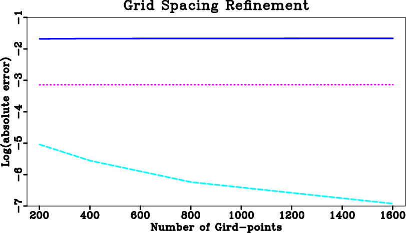
same model in Figure 1, we carry out both a source sampling refinement experiment and
a model grid spacing refinement experiment. The results are shown in Figures 4 and
5. Both figures are plotted for the traveltime at subsurface location ![]() km
for the source at location
km
for the source at location ![]() km. Although the curves vary for different locations, the source
sampling refinement experiment suggests the general need for approximately three times finer
source-sampling than that of Figure 2 to achieve the same level of accuracy.
km. Although the curves vary for different locations, the source
sampling refinement experiment suggests the general need for approximately three times finer
source-sampling than that of Figure 2 to achieve the same level of accuracy.

|
|---|
|
sfddiff
Figure 4. Source-sampling refinement experiment. The plot shows, at a fixed model grid sampling of |
|
|
|
|---|
|
gfddiff
Figure 5. Gird-spacing refinement experiment. The plot shows, at a fixed source sampling of |
|
|
Kirchhoff migration can use traveltime source-derivatives in two ways: for traveltime interpolation when
the source and receiver of a trace does not lie on the source grid of pre-computed traveltime tables,
and for anti-aliasing. Figure 6 shows a synthetic model of constant-velocity-gradient with
five dome-shaped reflectors. The model has a ![]() km grid spacing in both directions. We solve for
traveltimes and source-derivatives by the modified FMM introduced in Appendix A at 21 sparse shots of
uniform spacing 0.5 km, and migrate synthetic zero-offset data. The interpolation of source-derivative
for the anti-aliasing purpose follows the method described in Appendix B. 48 interpolations are carried
out within each sparse source sampling interval. Figures 7 and 8 compare
the images obtained by three different interpolations and the effect of anti-aliasing. All images are
plotted at the same scale. We do not limit migration aperture for all cases and adopt the anti-aliasing
criteria suggested by Abma et al. (1999) to filter the input trace before mapping a sample to the image, where
the source-derivative and receiver-derivative (in the zero-offset case they coincide) determine the filter
coefficients. As expected, the cubic Hermite interpolation with anti-aliasing leads to the most desirable
image. The image could be further improved by considering not only the kinematics predicted by the traveltimes
but also the amplitude factors (Vanelle et al., 2006; Dellinger et al., 2000).
km grid spacing in both directions. We solve for
traveltimes and source-derivatives by the modified FMM introduced in Appendix A at 21 sparse shots of
uniform spacing 0.5 km, and migrate synthetic zero-offset data. The interpolation of source-derivative
for the anti-aliasing purpose follows the method described in Appendix B. 48 interpolations are carried
out within each sparse source sampling interval. Figures 7 and 8 compare
the images obtained by three different interpolations and the effect of anti-aliasing. All images are
plotted at the same scale. We do not limit migration aperture for all cases and adopt the anti-aliasing
criteria suggested by Abma et al. (1999) to filter the input trace before mapping a sample to the image, where
the source-derivative and receiver-derivative (in the zero-offset case they coincide) determine the filter
coefficients. As expected, the cubic Hermite interpolation with anti-aliasing leads to the most desirable
image. The image could be further improved by considering not only the kinematics predicted by the traveltimes
but also the amplitude factors (Vanelle et al., 2006; Dellinger et al., 2000).

|
|---|
|
modl
Figure 6. Constant-velocity-gradient background model |
|
|

|
|---|
|
hzodmig
Figure 7. Zero-offset Kirchhoff migration image with (top) the cubic Hermite interpolation and (bottom) the shift interpolation. |
|
|

|
|---|
|
lzodmig
Figure 8. Zero-offset Kirchhoff migration image with (top) the linear interpolation and (bottom) the cubic Hermite interpolation without anti-aliasing. |
|
|
|
|
|
|
Kirchhoff migration using eikonal-based computation of traveltime source-derivatives |