Multichannel adaptive deconvolution based on streaming prediction-error filter

2D wedge model

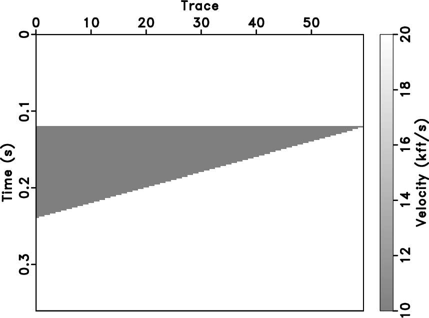
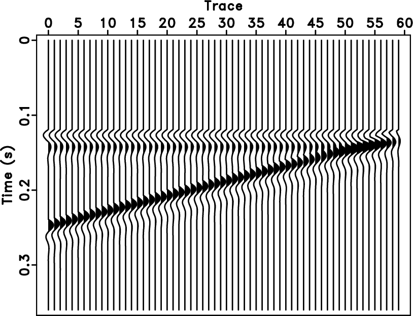
The second example is shown in figure 7a. We use a 2D benchmark wedge model to prove the necessity of the spatial constraint for the streaming PEF deconvolution. The velocity of the wedge in the model is 10 kft/s, and the velocity of the upper and lower media is 20 kft/s, therefore, the wave impedance corresponding to the top and bottom interfaces of the wedge are reversed. The minimum-phase wavelet with the dominant frequency of 30 Hz is selected to create the synthetic data (figure 7b), where the wavelet of the top and bottom interfaces appears interference started from the 45th trace. 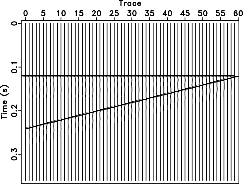The synthetic data are firstly processed using the traditional predictive deconvolution method (the filter length is 3) and the regularizednon-stationary autoregressive (RNA) method (the filter length is 3) based on the iterative algorithm (Liu and Fomel, 2011), and the deconvolution results are shown in figures 7c and  7d, respectively. 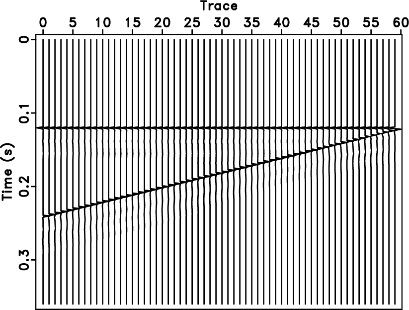Due to the model is stationary data, both methods can effectively improve the resolution and distinguish the top and bottom interfaces of the wedge model, but the traditional predictive deconvolution method is not suitable for processing nonstationary data (see figure 5) and iterative RNA deconvolution produces high computational cost. Then we design a streaming PEF with 3 (time) coefficients, the prediction step $\alpha=1$ , and the time constraint factor $\epsilon_t=0.2$ for each sample to further verify the effectiveness of the spatial constraint. Figures 7e and  7f show the streaming PEF deconvolution results without spatial constraint ( $\epsilon_x=0$ ) and with spatial constraint ( $\epsilon_x=0.5$ ), respectively. Both single-channel and multichannel deconvolution improve the vertical resolution, however, the result without spatial constraint appears with unstable fluctuation and spatial discontinuity, especially at rectangle location in figure 7e. The spatial constraint can effectively reduce the fluctuation and enhance the structural continuity of deconvolution result. Meanwhile, the computation time of the traditional method, iterative method, single-channel, and multichannel streaming PEF deconvolution method is 0.011 s, 0.220 s, 0.011 s, and 0.012 s, respectively.

wedge,wseis2,tpef,apef,spef0,spef1
Figure 7. Wedge model. Wedge velocity model (a), synthetic data (b), the result of traditional predictive deconvolution (c), the result of iterative deconvolution (d), the result of adaptive single-channel deconvolution without spatial constraint (e), the result of adaptive multichannel deconvolution with patial constraint (f).

Multichannel adaptive deconvolution based on streaming prediction-error filter