|
|
|
|
Multichannel adaptive deconvolution based on streaming prediction-error filter |
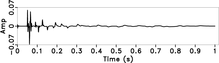
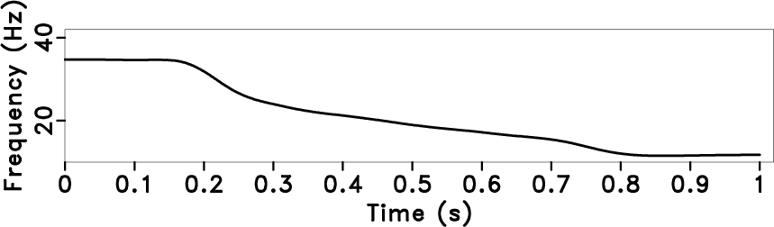
Next, we improve the adaptive deconvolution result by involving the
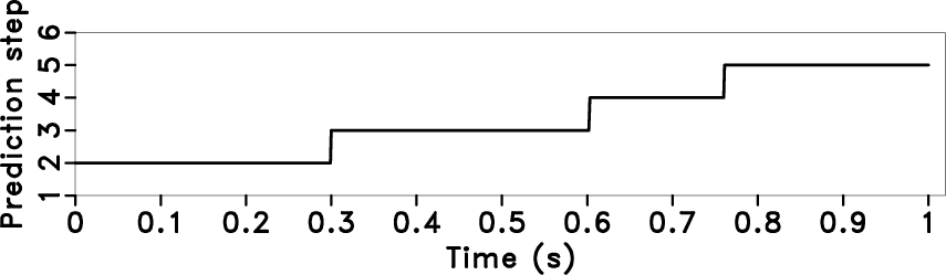
time-varying prediction step, and the result is shown in
figure 6.
Figures 6a and
6b show the decay of local frequency
and the time-varying prediction step by using equation 14
where ![]() , respectively. Figure 6c
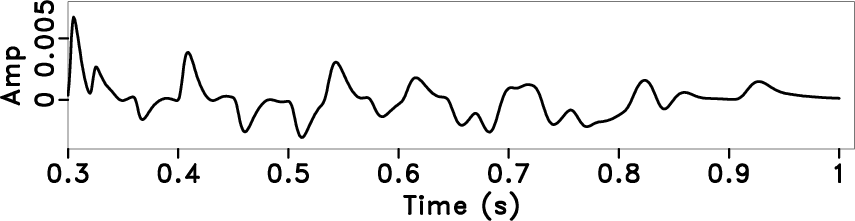
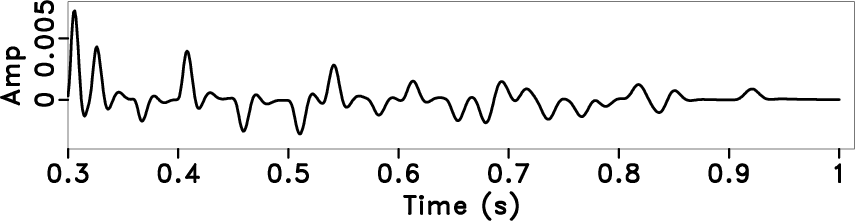
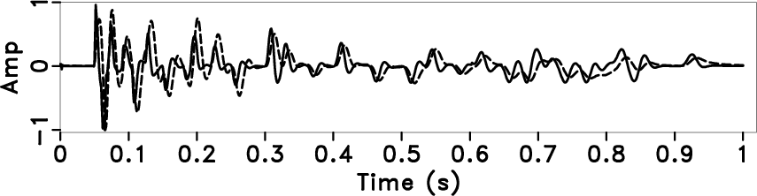
shows that the proposed method keeps the relative amplitude
relationship without auto gain correction (AGC) and the time
resolution is reasonably enhanced.
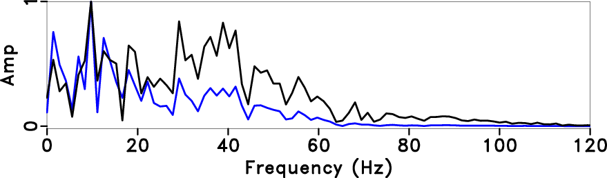
Figure 6d shows amplitude spectrum of
the synthetic data before and after deconvolution, where the grey line
is the original synthetic data and the black line is the deconvolution
result. It can be seen from figure 6d that the amplitude spectrum
broadens after the deconvolution.
, respectively. Figure 6c
shows that the proposed method keeps the relative amplitude
relationship without auto gain correction (AGC) and the time
resolution is reasonably enhanced.
Figure 6d shows amplitude spectrum of
the synthetic data before and after deconvolution, where the grey line
is the original synthetic data and the black line is the deconvolution
result. It can be seen from figure 6d that the amplitude spectrum
broadens after the deconvolution.
|
|---|
|
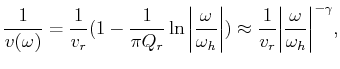
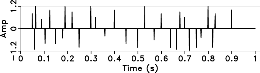
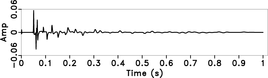
refl,in
Figure 4. A synthetic seismic trace example. The reflectivity (a), synthetic trace with Q attenuation (b). |
|
|
|
|---|
|
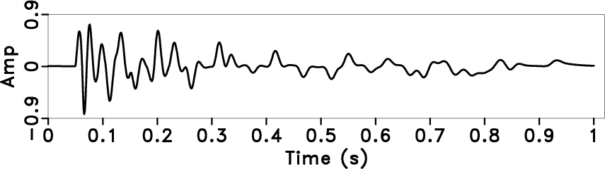
tpef,wtpef,spef0,wspef0
Figure 5. Deconvolution results by using different methods. Traditional predictive deconvolution (a), local display of (a) (b), streaming PEF deconvolution (c), local display of figure (c) (d). |
|
|
|
|---|
|
lfe,vlag0,nodif,zsdif
Figure 6. Deconvolution by using streaming PEF with time-varying prediction steps. Local frequency (a), time-varying prediction step (b), the deconvolution result with the proposed method (solid line), which is compared with the original trace (dotted line) (c), amplitude spectrum (The grey line is the original data, and the black line is the deconvolution result) (d). |
|
|
|
|
|
|
Multichannel adaptive deconvolution based on streaming prediction-error filter |