|
|
|
|
Multichannel adaptive deconvolution based on streaming prediction-error filter |
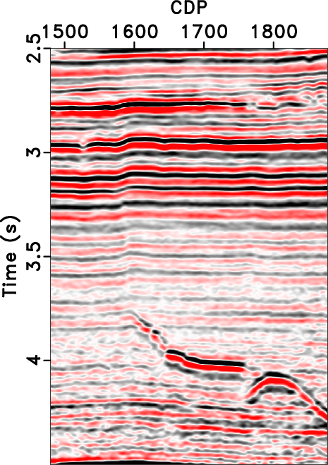
For the field data test, we use a 2D poststack section with time interval of
2 ms. The input is shown in figure 8a. For
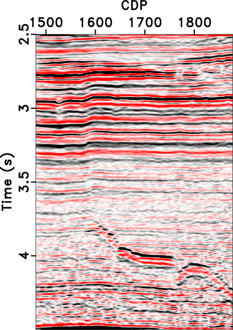
comparison, we apply the traditional predictive deconvolution (the filter
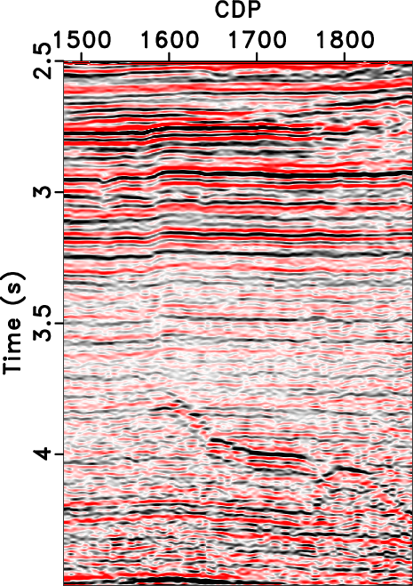
length is 6) and the iterative method (the filter length is 6) to enhance
the time resolution, as shown in figures 8b
and 8c.
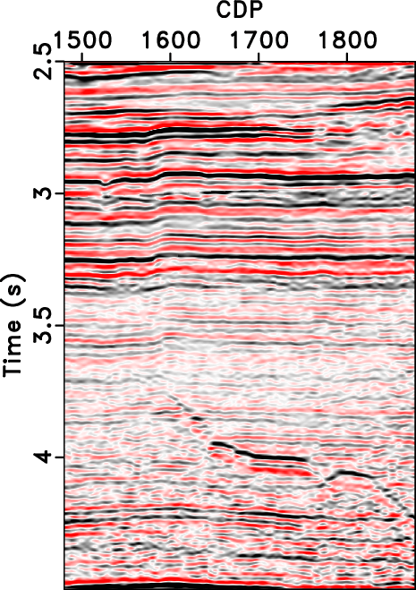
Figure 8d shows a processing result using
the proposed streaming PEF deconvolution method. The streaming PEF parameters
are 6 (![]() ), 0.032 (
), 0.032 (![]() ), 25000 (
), 25000 (
![]() ), and 10000 (
), and 10000 (
![]() ).
The computation time of traditional, iterative method, and streaming
PEF deconvolution methods are 0.024 s, 18.767 s, and 1.018 s, respectively,
however, the traditional deconvolution method cannot enhance the time
resolution at all time because of nonstationary of the field data. The
proposed deconvolution and iterative methods can improve the vertical
resolution at different times, so both methods are more suitable for
processing nonstationary data. Moreover, compared with the traditional
and iterative methods, the proposed method can better keep the
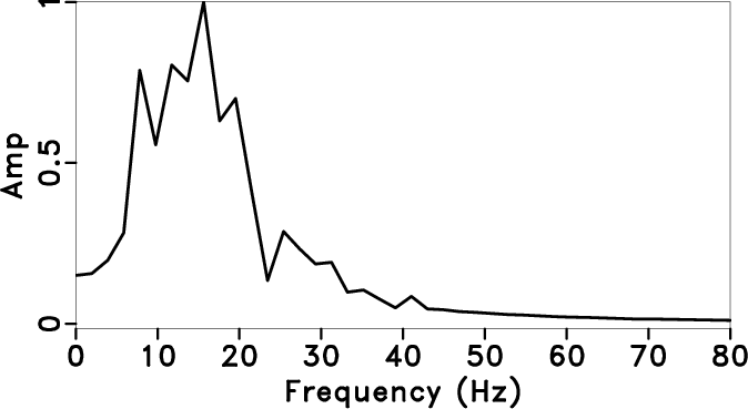
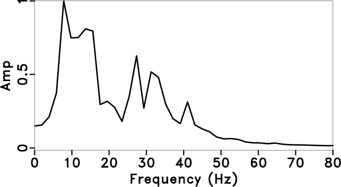
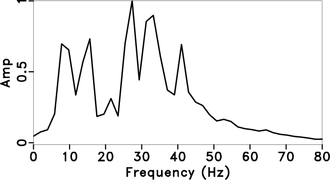
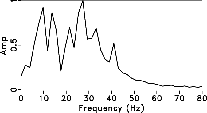
continuity of events. Furthermore, we select a part of the data near to the
reservoir layer from 3-3.5 s to calculate the average amplitude spectrum of
the data before and after deconvolution, as shown in
figure 9.
Figure 9 confirms that the average
amplitude spectrum of the seismic section after being processed by the
streaming PEF deconvolution is broader than that of the traditional
deconvolution result and slightly narrower than that of the iterative
deconvolution result in the effective frequency range. However, according to
the computation time of the different deconvolution methods, the
computational efficiency of the proposed method is significantly improved
compared with the iterative method. It further verifies the effectiveness
and high efficiency of the streaming PEF deconvolution method in processing
nonstationary seismic data.
).
The computation time of traditional, iterative method, and streaming
PEF deconvolution methods are 0.024 s, 18.767 s, and 1.018 s, respectively,
however, the traditional deconvolution method cannot enhance the time
resolution at all time because of nonstationary of the field data. The
proposed deconvolution and iterative methods can improve the vertical
resolution at different times, so both methods are more suitable for
processing nonstationary data. Moreover, compared with the traditional
and iterative methods, the proposed method can better keep the
continuity of events. Furthermore, we select a part of the data near to the
reservoir layer from 3-3.5 s to calculate the average amplitude spectrum of
the data before and after deconvolution, as shown in
figure 9.
Figure 9 confirms that the average
amplitude spectrum of the seismic section after being processed by the
streaming PEF deconvolution is broader than that of the traditional
deconvolution result and slightly narrower than that of the iterative
deconvolution result in the effective frequency range. However, according to
the computation time of the different deconvolution methods, the
computational efficiency of the proposed method is significantly improved
compared with the iterative method. It further verifies the effectiveness
and high efficiency of the streaming PEF deconvolution method in processing
nonstationary seismic data.
|
|---|
|
data,tpef,apef,vlag-spef
Figure 8. Deconvolution results by using different methods. Poststack field data (a), traditional predictive deconvolution (b), iterative deconvolution (c), streaming PEF deconvolution (d). |
|
|
|
|---|
|
zspec0,zspec1,zspec2,zspec3
Figure 9. Comparison of the average amplitude spectrum of the deconvolution results and original field data. Original field data (a), traditional predictive deconvolution (b), iterative deconvolution (c), streaming PEF deconvolution (d). |
|
|
|
|
|
|
Multichannel adaptive deconvolution based on streaming prediction-error filter |