|
|
|
|
Continuous time-varying Q-factor estimation method in the time-frequency domain |
The centroid frequency ![]() with respect to the amplitude spectrum
with respect to the amplitude spectrum ![]() can be defined as (Quan and Harris, 1997)
can be defined as (Quan and Harris, 1997)
The variance
![]() of the centroid frequency can be defined as
of the centroid frequency can be defined as
The time-frequency spectrum ![]() replaces the Fourier amplitude spectrum
replaces the Fourier amplitude spectrum
![]() in equations 1 and equations 2, and the
instantaneous centroid frequency
in equations 1 and equations 2, and the
instantaneous centroid frequency ![]() and instantaneous variance
and instantaneous variance
![]() of the amplitude spectrum are defined as
of the amplitude spectrum are defined as
The above equations show that the instantaneous centroid frequency and variance are calculated instantaneously using the amplitude spectrum information at a specific time. However, at times without effective spectrum information, reasonable results cannot be obtained using this calculation method.
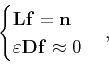
Fomel (2007a) defined the local attributes of the seismic signals such as local frequency and local similarity using shaping regularization. In this paper, we use a similar method to define the local centroid frequency and local variance. Equation 3 shows that the instantaneous centroid frequency is a division regarding two integrals and can be expressed in linear algebraic notation as
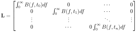 is a diagonal matrix composed of the denominators in equation 3.
Equation 5 can be regarded as an inversion problem. We use the
least-squares criterion to calculate
is a diagonal matrix composed of the denominators in equation 3.
Equation 5 can be regarded as an inversion problem. We use the
least-squares criterion to calculate
The theory of shaping regularization comes from data smoothing. It has
fewer parameters and a faster convergence speed than the traditional
Tikhonov regularization method. When considering shaping
regularization, the shaping operator
![]() can be defined as
can be defined as
The least-squares solution under the shaping regularization constraint can be obtained by substituting the above equation into equation 7
Similarly, the local variance
![]() can be
calculated using the above method. When calculating the local centroid
frequency, only one smoothing parameter is needed to control the
locality and smoothness of the local centroid frequency. The local
centroid frequency is not calculated instantaneously using the
information at a specific time or calculated globally in a time window
but is calculated locally using the information around the time. Thus,
a relatively reasonable local centroid frequency can be continuously
and smoothly calculated at the time of missing information (such as
when the amplitude spectrum is zero). In this paper, we use the local
centroid frequency to estimate the continuous time-varying Q values of
the formation.
can be
calculated using the above method. When calculating the local centroid
frequency, only one smoothing parameter is needed to control the
locality and smoothness of the local centroid frequency. The local
centroid frequency is not calculated instantaneously using the
information at a specific time or calculated globally in a time window
but is calculated locally using the information around the time. Thus,
a relatively reasonable local centroid frequency can be continuously
and smoothly calculated at the time of missing information (such as
when the amplitude spectrum is zero). In this paper, we use the local
centroid frequency to estimate the continuous time-varying Q values of
the formation.
|
|
|
|
Continuous time-varying Q-factor estimation method in the time-frequency domain |