Homework 6

Computational part

1. We start by returning to the model from Homeworks 1 and 5 with a hyperbolic reflector under a constant velocity layer. The model is shown in Figure 1. Now we will approach the imaging task using reverse-time migration with a two-way wave extrapolation. Figure 2a shows synthetic zero-offset data generated by Kirchhoff modeling. Figure 8 shows an image generated by zero-offset reverse-time migration using an explicit finite-difference wave extrapolation in time.

   Your task: Change the program for reverse-time migration to implement forward-time modeling using the ``exploding reflector'' approach.

   1. Change directory

      cd hw6/hyper
      

   2. Run

      scons view
      

      to generate figures and display them on your screen.
   3. Run

      scons wave.vpl
      

      to observe a movie of reverse-time wave extrapolation.
   4. Edit the program in the rtm.c file to implement a process opposite to migration: starting from the reflectivity image like the one in Figure 8 and generating zero-offset data like the one in Figure 2a.
   5. Run

      scons view
      

      again to observe the differences.

   

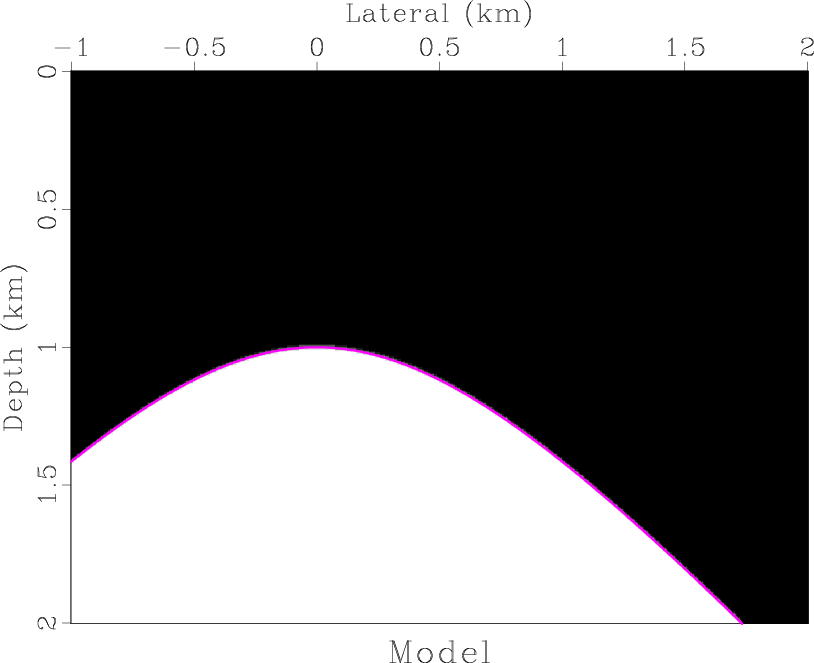
   model
   Figure 1. Synthetic velocity model with a hyperbolic reflector.

   

   
   

   

   data,image
   Figure 2. (a) Synthetic zero-offset data corresponding to the model in Figure 1. (b) Image generated by reverse-time exploding-reflector migration. The location of the exact reflector is indicated by a curve.

   

   
   

   from rsf.proj import *
   
   # Make a reflector model 
   Flow('refl',None,
        '''
        math n1=10001 o1=-4 d1=0.001 output="sqrt(1+x1*x1)" 
        ''')
   Flow('model','refl',
        '''
        window min1=-3 max1=3 j1=5  |
        unif2 n1=401 d1=0.005 v00=1,2 |
        put label1=Depth unit1=km label2=Lateral unit2=km |
        smooth rect1=3
        ''')
   
   Plot('model',
        '''
        window min2=-1 max2=2 |
        grey allpos=y bias=1 title=Model 
        ''')
   Plot('refl',
        '''
        graph wanttitle=n wantaxis=n yreverse=y
        min1=-1 max1=2 min2=0 max2=2 
        plotfat=3 plotcol=4 
        ''') 
   Result('model','model refl','Overlay')
   
   # Kirchoff zero-offset modeling
   Flow('dip','refl','math output="x1/input" ')
   
   Flow('data','refl dip',
        '''
        kirmod nt=1501 dt=0.004 freq=10
        ns=1201 s0=-3 ds=0.005 nh=1 dh=0.01 h0=0
        twod=y vel=1 dip=${SOURCES[1]} verb=y |
        window | costaper nw2=200 
        ''')
   Result('data',
        '''
        window min2=-2 max2=2 min1=1 max1=4 |
        grey title="Zero-Offset Data" grid=y 
        label1=Time unit1=s label2=Distance unit2=km
        ''')
   
   # Reverse-time migration
   proj = Project()
   prog = proj.Program('rtm.c')
   
   Flow('image wave','model %s data' % prog[0],
        '''
        pad beg1=200 end1=200 | math output=0.5 |
        ./${SOURCES[1]} data=${SOURCES[2]} 
        wave=${TARGETS[1]} jt=20 n0=200
        ''')
   
   # Display wave propagation movie
   Plot('wave',
        '''
        window min2=-1 max2=2 min1=0 max1=2 f3=33 |
        grey wanttitle=n gainpanel=all
        ''',view=1)
   
   # Display image
   Plot('image',
        '''
        window min2=-1 max2=2 min1=0 max1=2 |
        grey title=Image 
        ''')
   Result('image','image refl','Overlay')
   
   End()
   

   /* 2-D zero-offset reverse-time migration */
   #include <rsf.h>
   
   #ifdef _OPENMP
   #include <omp.h>
   #endif
   
   static int n1, n2;
   static float c0, c11, c21, c12, c22;
   
   static void laplacian(float **uin  /* [n2][n1] */, 
   		      float **uout /* [n2][n1] */)
   /* Laplacian operator, 4th-order finite-difference */
   {
       int i1, i2;
   
   #ifdef _OPENMP
   #pragma omp parallel for	                       private(i2,i1)		                       shared(n2,n1,uout,uin,c11,c12,c21,c22,c0)
   #endif	    
       for (i2=2; i2 < n2-2; i2++) {
   	for (i1=2; i1 < n1-2; i1++) {
   	    uout[i2][i1] = 
   		c11*(uin[i2][i1-1]+uin[i2][i1+1]) +
   		c12*(uin[i2][i1-2]+uin[i2][i1+2]) +
   		c21*(uin[i2-1][i1]+uin[i2+1][i1]) +
   		c22*(uin[i2-2][i1]+uin[i2+2][i1]) +
   		c0*uin[i2][i1];
   	}
       }
   }
   
   int main(int argc, char* argv[])
   {
       int it,i1,i2;        /* index variables */
       int nt,n12,n0,nx, jt;
       float dt,dx,dz, dt2,d1,d2;
   
       float  **vv, **dd;          
       float  **u0,**u1,u2,**ud; /* tmp arrays */
   
       sf_file data, imag, modl, wave; /* I/O files */
   
       /* initialize Madagascar */
       sf_init(argc,argv);
   
       /* initialize OpenMP support */ 
       omp_init();
   
       /* setup I/O files */
       modl = sf_input ("in");   /* velocity model */
       imag = sf_output("out");  /* output image */
    
       data = sf_input ("data"); /* seismic data */
       wave = sf_output("wave"); /* wavefield */
       
       /* Dimensions */
       if (!sf_histint(modl,"n1",&n1)) sf_error("n1");
       if (!sf_histint(modl,"n2",&n2)) sf_error("n2");
   
       if (!sf_histfloat(modl,"d1",&dz)) sf_error("d1");
       if (!sf_histfloat(modl,"d2",&dx)) sf_error("d2");
   
       if (!sf_histint  (data,"n1",&nt)) sf_error("n1");
       if (!sf_histfloat(data,"d1",&dt)) sf_error("d1");
   
       if (!sf_histint(data,"n2",&nx) || nx != n2) 
   	sf_error("Need n2=%d in data",n2);
   
       n12 = n1*n2;
   
       if (!sf_getint("n0",&n0)) n0=0;
       /* surface */
       if (!sf_getint("jt",&jt)) jt=1; 
       /* time interval */
   
       sf_putint(wave,"n3",1+(nt-1)/jt);
       sf_putfloat(wave,"d3",-jt*dt);
       sf_putfloat(wave,"o3",(nt-1)*dt);
   
       dt2 = dt*dt;
   
       /* set Laplacian coefficients */
       d1 = 1.0/(dz*dz);
       d2 = 1.0/(dx*dx);
   
       c11 = 4.0*d1/3.0;
       c12=  -d1/12.0;
       c21 = 4.0*d2/3.0;
       c22=  -d2/12.0;
       c0  = -2.0 * (c11+c12+c21+c22);
   
       /* read data and velocity */
       dd = sf_floatalloc2(nt,n2);
       sf_floatread(dd[0],nt*n2,data);
   
       vv = sf_floatalloc2(n1,n2);
       sf_floatread(vv[0],n12,modl);
   
       /* allocate temporary arrays */
       u0=sf_floatalloc2(n1,n2);
       u1=sf_floatalloc2(n1,n2);
       ud=sf_floatalloc2(n1,n2);
       
       for (i2=0; i2<n2; i2++) {
   	for (i1=0; i1<n1; i1++) {
   	    u0[i2][i1]=0.0;
   	    u1[i2][i1]=0.0;
   	    ud[i2][i1]=0.0;
   	    vv[i2][i1] *= vv[i2][i1]*dt2;
   	}
       }
   
       /* Time loop */
       for (it=nt-1; it >= 0; it-) {
   	sf_warning("%d;",it);
   
   	laplacian(u1,ud);
   
   #ifdef _OPENMP
   #pragma omp parallel for	         private(i2,i1,u2)		         shared(ud,vv,it,u1,u0,dd,n0)
   #endif
   	for (i2=0; i2<n2; i2++) {
   	    for (i1=0; i1<n1; i1++) {
   		/* scale by velocity */
   		ud[i2][i1] *= vv[i2][i1];
   
   		/* time step */
   		u2 = 
   		    2*u1[i2][i1] 
   		    - u0[i2][i1] 
   		    + ud[i2][i1]; 
   		
   		u0[i2][i1] = u1[i2][i1];
   		u1[i2][i1] = u2;
   	    }
   
   	    /* inject data */
   	    u1[i2][n0] += dd[i2][it];
   	}
   
   	if (0 == it%jt) 
   	    sf_floatwrite(u1[0],n12,wave);       
       }
       sf_warning(".");	
   
       /* output image */
       sf_floatwrite(u1[0],n12,imag);
       
       exit (0);
   }
   

2. Figure 3 shows the Sigsbee velocity model (Paffenholz et al., 2002) and its an approximate filtered reflectivity.

   

   zvel,zref
   Figure 3. (a) Sigsbee velocity model. (b) Approximate reflectivity of the Sigsbee model (an ideal image).

   

   
   

   Your task: Apply your exploding-reflector modeling and migration program from the previous task to generate zero-offset data for Sigsbee and image it.

   1. Change directory

      cd hw6/sigsbee
      

   2. Run

      scons view
      

      to generate figures and display them on your screen.
   3. Modify the SConstruct file to implement the modeling and migration experiment.
   4. Include your results in the paper by editing the hw6/paper.tex file.
   5. For EXTRA CREDIT, make sure that your modeling and migration are adjoint to each other and apply least-squares exploding-reflector reverse-time migration to the Sigsbee model.

   from rsf.proj import *
   
   # Download velocity model from the data server
   ##############################################
   vstr = 'sigsbee2a_stratigraphy.sgy'
   Fetch(vstr,'sigsbee')
   Flow('zvstr',vstr,'segyread read=data')
   
   Flow('zvel','zvstr',
        '''
        put d1=0.025 o2=10.025 d2=0.025
        label1=Depth unit1=kft label2=Lateral unit2=kft |
        scale dscale=0.001
        ''')
   
   Result('zvel',
          '''
          window f1=200 |
          grey title=Velocity titlesz=7 color=j
          screenratio=0.3125 screenht=4 labelsz=5
          mean=y
          ''')
   
   # Compute approximate reflectivity
   ##################################
   Flow('zref','zvel',
        '''
        depth2time velocity=$SOURCE nt=2501 dt=0.004 |
        ai2refl | ricker1 frequency=10 |
        time2depth velocity=$SOURCE
        ''')
   
   Result('zref',
          '''
          window f1=200 |
          grey title=Reflectivity titlesz=7
          screenratio=0.3125 screenht=4 labelsz=5
          ''')
   
   End()
   

3. In the last part of the homework, you will work with a field dataset: a 2-D line from the Blake Outer Ridge area offshore Florida and Georgia (Figure 4). It was collected by USGS in order to study the occurrence of methane hydrates. The presence of gas hydrates is manifested by a so-called BSR (bottom-simulating reflector). The dataset and its analysis for gas hydrate detection are described by Ecker et al. (2000,1998).

   map2 Figure 4. Map of the Blake Outer Ridge area. An region of known gas hydrate distribution as mapped from seismic bottom simulating reflectors (BSR) is highlighted. The seismic survey area is marked by a rectangle.

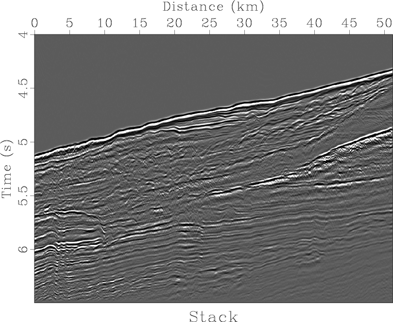
   The following figures show the dataset at different stages of seismic data processing: from initial data to an image in depth.

   Your task: Modify the data processing sequence to create a justifiably better image.

   

   nmo
   Figure 5. Common midpoint gather (left), velocity analysis panel using normal moveout (middle), and common midpoint gather after normal moveout (right). A curve in the middle plot indicates an automatically picked velocity trend.

   

   
   

   

   noff,stack
   Figure 6. (a) Near-offset section. (b) Normal moveout stack.

   

   
   

   

   picks,vel
   Figure 7. (a) Picked stacking velocity. (b) Interval velocity estimated by Dix inversion.

   

   
   

   

   image
   Figure 8. Seismic image created by converting stacked data from time to depth. Can you identify geological features that are not properly imaged?

   

   
   

   from rsf.proj import *
   
   # get data
   Fetch('cmps-tp.HH','blake')
   
   # CMP (common midpoint) gathers
   Flow('cmps','cmps-tp.HH',
        'dd form=native | reverse which=2')
   # one CMP
   Flow('cmp','cmps',
        '''
        window f3=950 n3=1 max1=6 |
        put o2=0.0 d2=1
        ''')
   Plot('cmp',
        '''
        grey title="CMP gather" 
        unit1=s label2=Offset unit2=km
        ''')
   
   # Near-offset section
   Result('noff','cmps',
          '''
          window n2=1 n3=1024 |
          grey title="Near Offset Section" 
          unit1=s label2=Distance unit2=km
          ''')
   
   # offset maps
   Flow('off1',None,'math n1=24 o1=0.4 d1=0.1  output=x1')
   Flow('off2',None,'math n1=24 o1=2.8 d1=0.05 output=x1')
   Flow('off','off1 off2','cat axis=1 ${SOURCES[1]}')
   Flow('offs','off','spray n=111')
   
   # Velocity analysis
   ###################
   
   vscan = '''
   vscan offset=${SOURCES[1]} 
   v0=1.4 nv=61 dv=0.005 half=n semblance=y
   '''
   pick = 'pick rect1=20 rect2=3 vel0=1.5'
   
   # compute semblance for one CMP
   Flow('vscan','cmp off',vscan)
   Plot('vscan',
        '''
        grey color=j allpos=y title="Velocity Scan" 
        unit1=s label2=Velocity unit2=km/s pclip=100
        ''')
   
   # pick maximum semblance for one CMP
   Flow('pick','vscan',pick)
   Plot('pick0','pick',
        '''
        graph transp=y yreverse=y min2=1.4 max2=1.7 
        plotcol=7 plotfat=10 pad=n wanttitle=n wantaxis=n
        ''')
   Plot('pick1','pick',
        '''
        graph transp=y yreverse=y min2=1.4 max2=1.7 
        plotcol=0 plotfat=1 pad=n wanttitle=n wantaxis=n
        ''')
   Plot('vscan2','vscan pick0 pick1','Overlay')
   
   # compute semblance for every 10th CMP
   Flow('vscans','cmps offs','window j3=10 | ' + vscan)
   
   # pick max semblance for every 10th CMP
   Flow('picks0','vscans',pick)
   
   # interpolate picks on the original grid
   Flow('picks','picks0',
        'transp | remap1 n1=1105 d1=0.05 o1=0 | transp')
   Result('picks',
          '''
          grey color=j scalebar=y barreverse=y 
          allpos=y bias=1.4
          title="Stacking Velocity" 
          label1=Time unit1=s label2=Distance unit2=km
          ''')
   
   # Normal moveout and stack
   ##########################
   
   nmo = '''
   nmo offset=${SOURCES[1]} 
   velocity=${SOURCES[2]} half=n
   '''
   
   Flow('nmo','cmp off pick',nmo)
   Plot('nmo',
        '''
        grey title="Normal Moveout" 
        unit1=s label2=Offset unit2=km
        ''')
   Result('nmo','cmp vscan2 nmo','SideBySideAniso')
   
   Flow('nmos','cmps off picks',nmo)
   Flow('stack','nmos','stack')
   Result('stack',
          '''
          window n2=1024 |
          grey title=Stack 
          unit1=s label2=Distance unit2=km
          ''')
   
   # Convert from time to depth
   ############################
   
   # Dix inversion
   Flow('semb','vscans picks0','slice pick=${SOURCES[1]}')
   Flow('vel0','picks0 semb',
        'dix rect1=20 rect2=2 weight=${SOURCES[1]}')
   
   # interpolate on the original grid
   Flow('vel','vel0',
        'transp | remap1 n1=1105 d1=0.05 o1=0 | transp')
   Result('vel',
          '''
          grey color=j scalebar=y barreverse=y 
          allpos=y bias=1.4
          title="Interval Velocity" 
          label1=Time unit1=s label2=Distance unit2=km
          ''')
   
   Flow('image','stack vel',
        '''
        time2depth velocity=${SOURCES[1]} 
        intime=y dz=0.005 nz=1001
        ''')
   Result('image',
          '''
          window n2=1024 min1=3 | grey title=Image
          label1=Depth unit1=km label2=Distance unit2=km
          ''')
   
   End()
   

   1. Change directory

      cd hw6/blake
      

   2. Run

      scons view
      

      to generate figures and display them on your screen.
   3. Modify the SConstruct file. Check your results by running

      scons view
      

      again.

Homework 6