Homework 5

Natural patterns

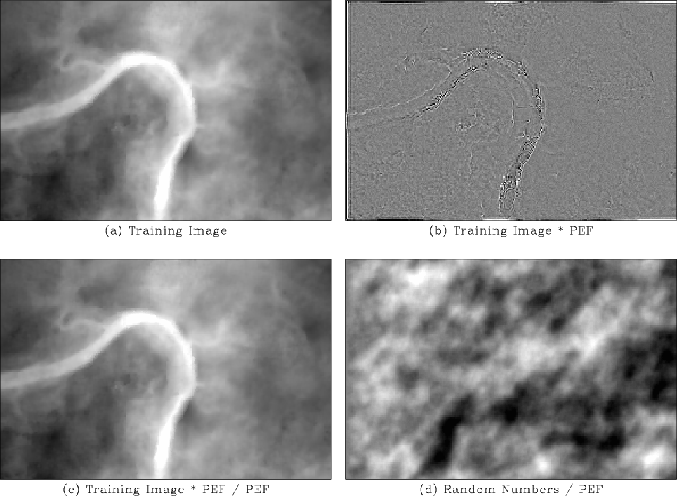
In this section we will extract multidimensional spatial patterns from natural images using the method of Claerbout and Brown (1999). Four examples, shown in Figures 1-4, contain:

1. Seismic horizon slice.
2. A slice from a CT-scan of a rock sample.
3. A remote-sensing satellite image.
4. Your own data (to be replaced by you).

In each of the cases, we follow the same workflow:

1. Remove a linear trend from the data.
2. Estimate a multi-dimensional prediction-error filter (PEF) on a helix.
3. Apply the inverse of the estimated PEF to random normally-distributed numbers to create a random spatial texture, which shares the covariance with the input.

horizon
Figure 1. Pattern extraction from a seismic time horizon.

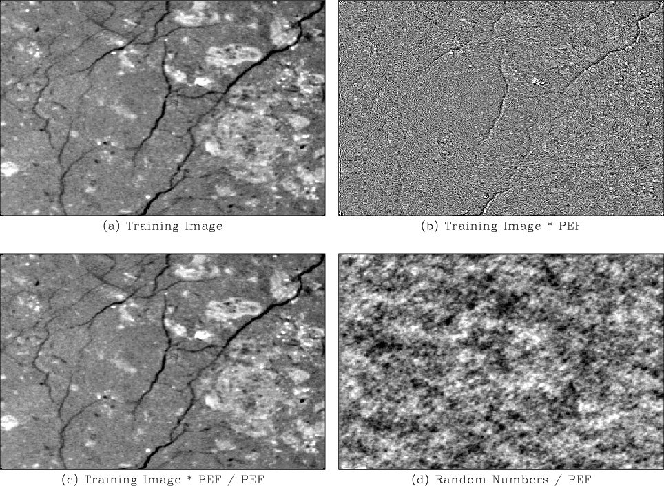
square
Figure 2. Pattern extraction from a CT-scan of a rock sample.

sat
Figure 3. Pattern extraction from a satellite image.

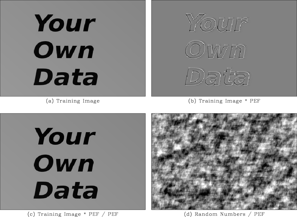
your
Figure 4. Pattern extraction from your own data.

from rsf.proj import *

g = 'grey crowd1=0.96 crowd2=0.85 wantaxis=n title="%s" '

# Seismic horizon
Fetch('horizon.asc','hall')
Flow('horizon','horizon.asc',
     '''
     echo in=$SOURCE data_format=ascii_float n1=3 n2=57036 | 
     dd form=native | window n1=1 f1=-1 | 
     put 
     n2=291 o2=35.031 d2=0.01 label2=y unit2=km 
     n1=196 o1=33.139 d1=0.01 label1=x unit1=km
     ''')

# CT-scan slice
Fetch('slice.rsf','ctscan')
Flow('circle','slice','dd type=float')
Flow('square','circle',
     'window window n1=366 n2=366 f1=73 f2=73')

# Satellite data
Fetch('mod.dat','ying')
Flow('sat','mod.dat',
     '''
     echo in=$SOURCE n1=1200 n2=1200 n3=7
     data_format=native_int |
     put d1=1 d2=1 o1=0 o2=0 d3=1 o3=0 |
     window n3=1 f3=3 | dd type=float |
     scale axis=2
     ''', stdin=0)

# Your own data
Fetch('your.dat','ying')
Flow('your','your.dat','dd type=float')

textures = ('horizon','square','sat','your')

for txt in textures:
    # Remove trend
    #-------
    m = txt+'-one'
    x = txt+'-x'
    y = txt+'-y'
    Flow(m,txt,'math output=1')
    Flow(x,txt,'math output=x1 | scale axis=2')
    Flow(y,txt,'math output=x2 | scale axis=2')
    flt = txt+'-flt'
    trd = txt+'-trd'
    Flow([flt,trd],[m,x,y,txt],
         '''
         cat ${SOURCES[1:3]} | 
         lpf match=${SOURCES[3]} pred=${TARGETS[1]}
         rect1=1000 rect2=1000 
         ''')
    t = txt+'-dtrd'
    Flow(t,[txt,trd],'add scale=1,-1 ${SOURCES[1]}')

    # Original
    #-----
    Plot(t,g % '(a) Training Image')

    # Estimate PEF
    #-------
    pef = txt+'-pef'
    lag = txt+'-lag'
    Flow([pef,lag],t,
         'hpef niter=50 a=10,10 lag=${TARGETS[1]}')

    # PEF residual
    #-------
    wht = txt+'-wht'
    Flow(wht,[t,pef],'helicon filt=${SOURCES[1]}')
    Plot(wht,g % '(b) Training Image * PEF')

    # Reconstruct original
    #-----------
    rec = txt+'-rec'
    Flow(rec,[wht,pef],'helicon filt=${SOURCES[1]} div=y')
    Plot(rec,g % '(c) Training Image * PEF / PEF')

    # Synthesized image
    #---------
    syn = txt+'-syn'
    Flow(syn,[t,pef],
              '''
              noise rep=y seed=2014 | 
              helicon filt=${SOURCES[1]} div=y
              ''')
    Plot(syn,g % '(d) Random Numbers / PEF')

    Result(txt,[t,wht,rec,syn],'TwoRows')

End()

Your task:

1. Change directory to hw5/pattern
2. Run

   scons view
   

   to reproduce the figures on your screen.
3. Modify the SConstruct file to replace Figure 4 with the figure containing your own data.
4. Why does the method fail in extracting some of the patterns? Did it succeed in extracting patterns from your data?

Homework 5