|
|
|
|
Homework 5 |
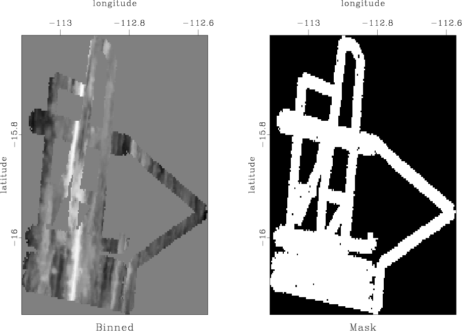
SeaBeam is an apparatus for measuring water depth both directly under a boat and somewhat off to the sides of the boat's track. In this part of the assignment, we will use a benchmark dataset from Claerbout (2014): SeaBeam data from a single day of acquisition. The original data are shown in Figure 5a.
|
|---|
|
seabeam0
Figure 5. (a) Water depth measurements from one day of SeaBeam acquisition. (b) Mask for locations of known data. |
|
|
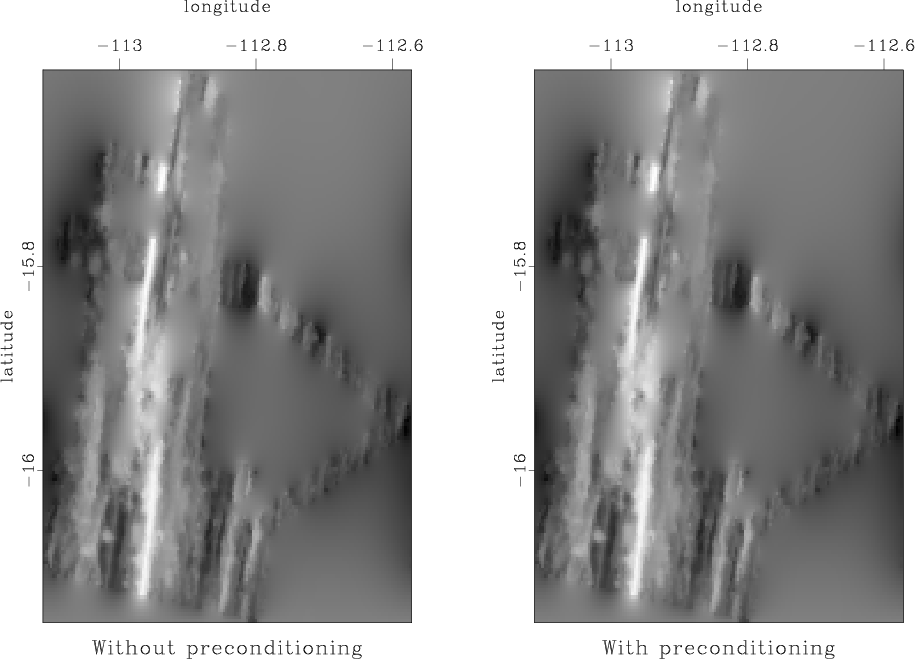
Program interpolate.c implements two alternative methods: regularized inversion using convolution with a multi-dimensional filter and preconditioning, which uses the inverse operation (recursive deconvolution or polynomial division on a helix) for model reparameterization.
Our first attempt is to use the Laplacian-factor filter from the previous homework. The results from the two methods are shown in Figure 6. They are not very successful in hiding the ``acquisition footprint''.
|
|---|
|
lseabeam
Figure 6. Left: missing data interpolation using regularization by convolution with a Laplacian factor. Right: missing data interpolation using model reparameterization by deconvolution (polynomial division) with a Laplacian factor. |
|
|
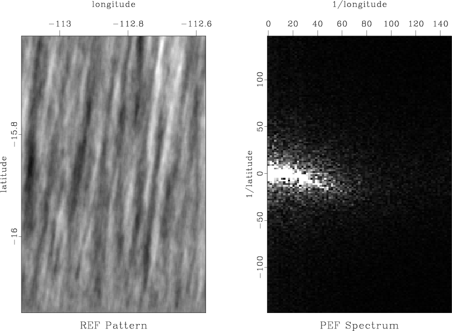
Next, we will try to estimate the model covariance from the available data. The covariance can be estimated using the prediction-error filter (PEF) method (Claerbout and Brown, 1999). A random realizations of the model pattern using this methods is shown in Figure 7.
|
|---|
|
rand
Figure 7. Left: data pattern generated using PEF method for inverse covariance estimation. Right: its Fourier spectrum. |
|
|
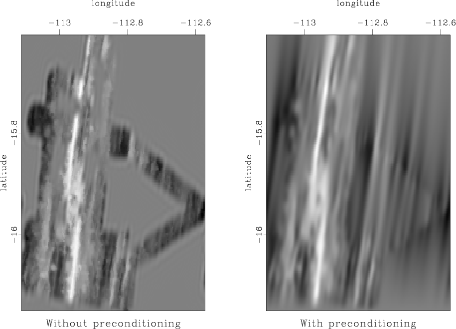
Our new attempt to interpolate missing data using the helical prediction-error filter is shown in Figure 8.
|
|---|
|
seabeam
Figure 8. Left: missing data interpolation using regularization by convolution with a prediction-error filter. Right: missing data interpolation using model reparameterization by deconvolution (polynomial division) with a prediction-error filter. |
|
|
/* Multi-dimensional missing data interpolation. */

#include <rsf.h>

int main(int argc, char* argv[])
{
    int na,ia, niter, n,i;
    float a0, *mm, *zero;
    bool prec, *known;
    char *lagfile;
    sf_filter aa;
    sf_file in, out, filt, lag, mask;

    sf_init (argc,argv);
    in = sf_input("in");
    filt = sf_input("filt");
    /* filter for inverse model covariance */
    out = sf_output("out");

    n = sf_filesize(in);

    if (!sf_getbool("prec",&prec)) prec=true;
    /* If y, use preconditioning */
    if (!sf_getint("niter",&niter)) niter=100;
    /* Number of iterations */

    if (!sf_histint(filt,"n1",&na)) sf_error("No n1=");
    aa = sf_allocatehelix (na);

    if (!sf_histfloat(filt,"a0",&a0)) a0=1.;

    /* Get filter lags */
    if (NULL == (lagfile = sf_histstring(filt,"lag"))) {
	for (ia=0; ia < na; ia++) {
	    aa->lag[ia]=ia+1;
	}
    } else {
	lag = sf_input(lagfile);
	sf_intread(aa->lag,na,lag);
	sf_fileclose(lag);
    }

    /* Get filter values */
    sf_floatread(aa->flt,na,filt);
    sf_fileclose(filt);

    /* Normalize */
    for (ia=0; ia < na; ia++) {
	aa->flt[ia] /= a0;
    }

    mm = sf_floatalloc(n);
    zero = sf_floatalloc(n);
    known = sf_boolalloc(n);

    /* specify known locations */
    mask = sf_input("mask");
    sf_floatread(mm,n,mask);
    sf_fileclose(mask);

    for (i=0; i < n; i++) {
	known[i] = (bool) (mm[i] != 0.0f);
	zero[i] = 0.0f;
    }

    /* Read input data */
    sf_floatread(mm,n,in);

    if (prec) {
	sf_mask_init(known);
	sf_polydiv_init(n, aa);
	sf_solver_prec(sf_mask_lop, sf_cgstep, sf_polydiv_lop,
		       n, n, n, mm, mm, niter, 0., "end");
    } else {
	sf_helicon_init(aa);
	sf_solver (sf_helicon_lop, sf_cgstep, n, n, mm, zero,
		   niter, "known", known, "x0", mm, "end");
    }

    sf_floatwrite(mm,n,out);

    exit (0);
}
|
from rsf.proj import *

# Download data
Fetch('apr18.h','seab')
Flow('data','apr18.h','dd form=native')

def grey(title):
    return '''
    grey pclip=100 labelsz=10 titlesz=12
    transp=n yreverse=n
    label1=longitude label2=latitude title="%s"
    ''' % title

def sgrey(title):
    return '''
    grey labelsz=10 titlesz=12 allpos=y
    transp=n yreverse=n title="%s"
    label1=1/longitude label2=1/latitude
    ''' % title

# Bin to regular grid
Flow('bin','data',
     '''
     window n1=1 f1=2 | math output='(2978-input)/387' |
     bin head=$SOURCE niter=150 nx=160 ny=160 xkey=0 ykey=1
     ''')

# Mask for known data
Flow('msk','bin',
     '''
     math output="abs(input)" |
     mask min=0.001 | dd type=float
     ''')

Plot('bin',grey('Binned'))
Plot('msk',grey('Mask') + ' allpos=y')

Result('seabeam0','bin msk','SideBySideAniso')

# Laplacian factorization

Flow('lag0.asc',None,
     '''
     echo 1 160 n1=2 n=160,160
     data_format=ascii_int in=$TARGET
     ''')
Flow('lag0','lag0.asc','dd form=native')

Flow('flt0.asc','lag0',
     '''
     echo -1 -1 a0=2 n1=2 lag=$SOURCE
     data_format=ascii_float in=$TARGET
     ''',stdin=0)
Flow('flt0','flt0.asc','dd form=native')

Flow('lapflt laplag','flt0',
     'wilson eps=1e-3 lagout=${TARGETS[1]}')

# Missing data interpolation with Laplacian

niter=100

program = Program('interpolate.c')

for prec in (0,1):
    interp='linterp%d' % prec
    Flow(interp,'bin msk lapflt %s' % program[0],
         '''
         ./${SOURCES[3]} prec=%d niter=%d
         mask=${SOURCES[1]} filt=${SOURCES[2]}
         ''' % (prec,niter))
    Plot(interp,grey('%s preconditioning' %
                     ('Without','With')[prec]))
Result('lseabeam','linterp0 linterp1','SideBySideAniso')

# Random realization of white noise
seed = 112018  # CHANGE ME!!!

Flow('white','bin',
     '''
     noise rep=y seed=%d var=0.02
     ''' % seed)

# Estimate PEF
Flow('pef lag','bin msk',
     '''
     hpef maskin=${SOURCES[1]} lag=${TARGETS[1]}
     a=5,3 niter=50
     ''')

Flow('rand','white pef',
     'helicon filt=${SOURCES[1]} div=y')
Plot('rand',grey('REF Pattern'))

Flow('frand','rand','spectra2')
Plot('frand',sgrey('PEF Spectrum'))

Result('rand','rand frand','SideBySideAniso')

# Missing data interpolation with PEF

niter=20 # CHANGE ME!!!

for prec in (0,1):
    interp='interp%d' % prec
    Flow(interp,'bin msk pef %s' % program[0],
         '''
         ./${SOURCES[3]} prec=%d niter=%d
         mask=${SOURCES[1]} filt=${SOURCES[2]}
         ''' % (prec,niter))
    Plot(interp,grey('%s preconditioning' %
                     ('Without','With')[prec]))
Result('seabeam','interp0 interp1','SideBySideAniso')

End()
|
Your task:
scons viewto reproduce the figures on your screen.
|
|
|
|
Homework 5 |