The helical coordinate

Examples of simple 2-D recursive filters

Let us associate $x$ - and $y$ -derivatives with a finite-difference stencil or template. (For simplicity take $\Delta x=\Delta y=1$ .)

$${\partial \over \partial x } \eq \begin{array}{\vert c\vert c\vert} \hline 1 & -1 \hline \end{array}$$ (3)

$${\partial \over \partial y } \eq \begin{array}{\vert r\vert} \hline 1 \hline -1 \hline \end{array}$$ (4)

Convolving a data plane with the stencil (3) forms the $x$ -derivative of the plane. Convolving a data plane with the stencil (4) forms the $y$ -derivative of the plane. On the other hand, deconvolving with (3) integrates data along the $x$ -axis for each $y$ . Likewise, deconvolving with (4) integrates data along the $y$ -axis for each $x$ . Next we look at a fully two-dimensional operator (like the cross derivative $\partial_{xy}$ ).

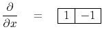
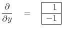
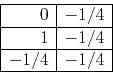
A nontrivial two-dimensional convolution stencil is

$$\begin{array}{\vert r\vert r\vert} \hline 0 & -1/4 \hline 1 & -1/4 \hline -1/4 & -1/4 \hline \end{array}$$ (5)

We will convolve and deconvolve a data plane with this operator. Although everything is shown on a plane, the actual computations are done in one dimension with equations (1) and (2). Let us manufacture the simple data plane shown on the left in Figure 3. Beginning with a zero-valued plane, we add in a copy of the filter (5) near the top of the frame. Nearby add another copy with opposite polarity. Finally add some impulses near the bottom boundary. The second frame in Figure 3 is the result of deconvolution by the filter (5) using the one-dimensional equation (2). Notice that deconvolution turns the filter itself into an impulse, while it turns the impulses into comet-like images. The use of a helix is evident by the comet images wrapping around the vertical axis.

wrap-four
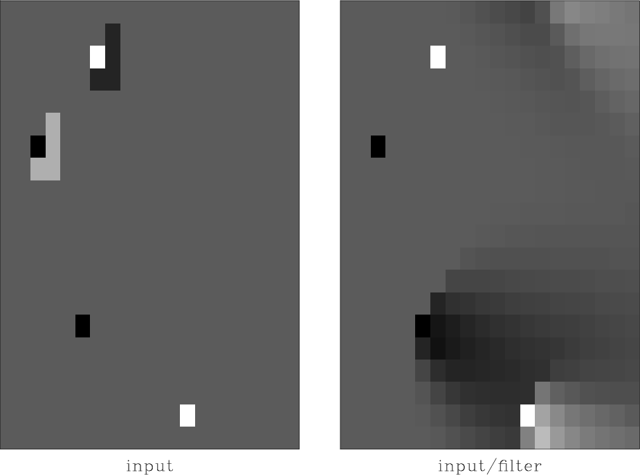
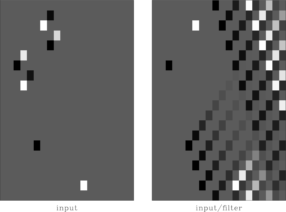
Figure 3. Illustration of 2-D deconvolution. Left is the input. Right is after deconvolution with the filter (5) as preformed by by module polydiv

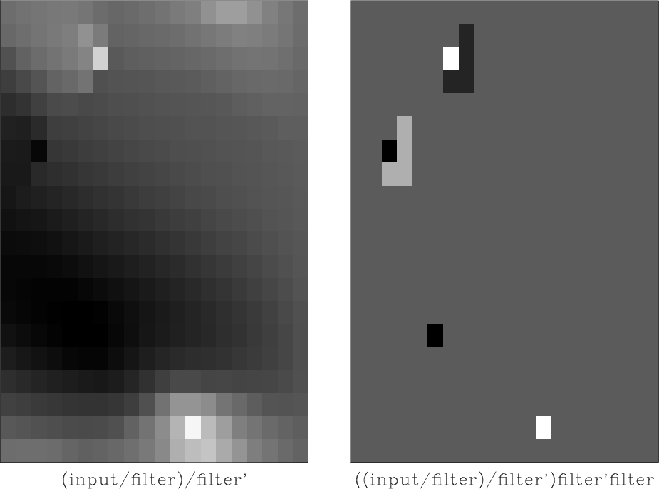
The filtering in Figure 3 ran along a helix from left to right. Figure 4 shows a second filtering running from right to left. Filtering in the reverse direction is the adjoint. After deconvolving both ways, we have accomplished a symmetical smoothing. The final frame undoes the smoothing to bring us exactly back to where we started. The smoothing was done with two passes of deconvolution and it is undone by two passes of convolution. No errors, no evidence remains of any of the boundaries where we have wrapped and truncated.

back-four
Figure 4. Recursive filtering backwards (leftward on the space axis) is done by the adjoint of 2-D deconvolution. Here we see that 2-D deconvolution compounded with its adjoint is exactly inverted by 2-D convolution and its adjoint.

Chapter explains the important practical role to be played by a multidimensional operator for which we know the exact inverse. Other than multidimensional Fourier transformation, transforms based on polynomial multiplication and division on a helix are the only known easily invertible linear operators.

In seismology we often have occasion to steer summation along beams. Such an impulse response is shown in Figure 6.

wrap-waves
Figure 5. A simple low-order 2-D filter whose inverse contains plane waves of two different dips. One of them is spatially aliased.

Of special interest are filters that destroy plane waves. The inverse of such a filter creates plane waves. Such filters are like wave equations. A filter that creates two plane waves is illustrated in figure 5.

dip
Figure 6. A simple low-order 2-D filter whose inverse times its inverse adjoint, is approximately a dipping seismic arrival.

The helical coordinate