Next: Multidimensional deconvolution breakthrough
Up: FILTERING ON A HELIX
Previous: FILTERING ON A HELIX
Convolution is the operation we do on polynomial coefficients
when we multiply polynomials.
Deconvolution is likewise for polynomial division.
Often, these ideas are described
as polynomials in the variable  .
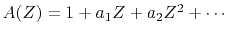
Take
.
Take  to denote the polynomial
with coefficients being samples of input data,
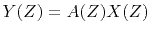
and let
to denote the polynomial
with coefficients being samples of input data,
and let  likewise denote the filter.
The convention I adopt here is that the first coefficient
of the filter has the value +1, so the filter's polynomial
is
likewise denote the filter.
The convention I adopt here is that the first coefficient
of the filter has the value +1, so the filter's polynomial
is
 .
To see how to convolve, we now identify the coefficient
of
.
To see how to convolve, we now identify the coefficient
of  in the product
 .
The usual case (
.
The usual case ( larger than the number
  of filter coefficients) is:
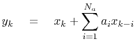 |
(1) |
Convolution computes  from
from  , whereas, deconvolution
(also called back substitution) does the reverse.
Rearranging (1); we get:
, whereas, deconvolution
(also called back substitution) does the reverse.
Rearranging (1); we get:
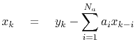 |
(2) |
where now, we are finding the output
from
its past outputs  and the present input
.
We see that the deconvolution process is essentially
the same as the convolution process,
except that the filter coefficients
are used with opposite polarity;
and the coefficients are applied to the past outputs
instead of the past inputs.
Needing past outputs is why deconvolution must be done sequentially
while convolution can be done in parallel.
and the present input
.
We see that the deconvolution process is essentially
the same as the convolution process,
except that the filter coefficients
are used with opposite polarity;
and the coefficients are applied to the past outputs
instead of the past inputs.
Needing past outputs is why deconvolution must be done sequentially
while convolution can be done in parallel.
Next: Multidimensional deconvolution breakthrough
Up: FILTERING ON A HELIX
Previous: FILTERING ON A HELIX
2015-03-25