The helical coordinate

Improving low-frequency behavior

It is nice having the 2-D helix derivative, but we can imagine even nicer 2-D low-cut filters. In 1-D, we designed a filter with an adjustable parameter, a cutoff frequency. In 1-D, we compounded a first derivative (which destroys low frequencies) with a leaky integration (which undoes the derivative at all other frequencies). The analogous filter in 2-D would be $-\nabla^2 /(-\nabla^2 + k_0^2)$ , which would first be expressed as a finite difference $(-Z^{-1} + 2.00 - Z) / (-Z^{-1} + 2.01 - Z)$ and then factored as we did the helix derivative.

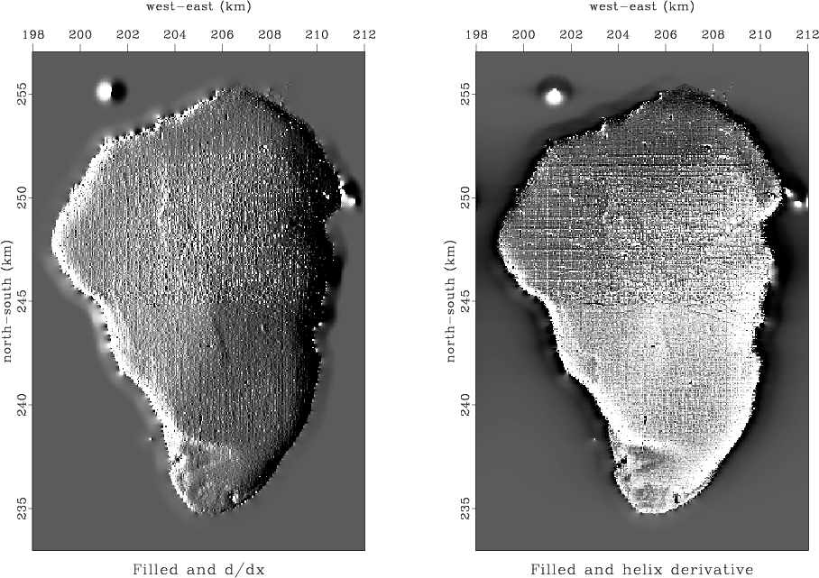
helgal
Figure 12. Galilee roughened by gradient and by helical derivative.

We can visualize a plot of the magnitude of the 2-D Fourier transform of the filter equation (13). It is a 2-D function of $k_x$ and $k_y$ and it should resemble $k_r=\sqrt{k_x^2 + k_y^2}$ . The point of the cone $k_r=\sqrt{k_x^2 + k_y^2}$ becomes rounded by the filter truncation, so $k_r$ does not reach zero at the origin of the $(k_x,k_y)$ -plane. We can force it to vanish at zero frequency by subtracting .183 from the lead coefficient 1.791. I did not do that subtraction in Figure 12, which explains the whiteness in the middle of the lake. I gave up on playing with both $k_0$ and filter length; and now, merely play with the sum of the filter coefficients.

The helical coordinate