The helical coordinate

FACTORED LAPLACIAN == HELIX DERIVATIVE

I had learned spectral factorization as a method for single seismograms. After I learned it, every time I saw a positive function I would wonder if it made sense to factor it. When total field magnetometers were invented, I found it as a way to deduce vertical and horizontal magnetic components. A few pages back, you saw how to use factorization to deduce the waveform passing through an absorptive medium. Then, we saw how the notion of ``impulse response'' applies not only to signals, but allows use of random noise on the sun to deduce the 3-D impulse response there. But the most useful application of spectral factorization so far is what comes next, factoring the Laplace operator, $-\nabla^2$ . Its Fourier transform $-((ik_x)^2+(ik_y)^2) \ge 0$ is positive, so it is a spectrum. The useful tool we uncover I dub the ``helix derivative.''

The signal:

$$\bold r \eq -\nabla^2 \eq \begin{array}{\vert r\vert r\vert r\ver... ...\vert r\vert} \hline -1&0&\cdots&0&-1&4&-1&0& \cdots&0&-1 \\ \hline \end{array}$$ (10)

is an autocorrelation function, because it is symmetrical about the ``4,'' and the Fourier transform of $-\nabla^2$ is $-((ik_x)^2+(ik_y)^2) \ge 0$ , which is positive for all frequencies $(k_x,k_y)$ . Kolmogoroff spectral-factorization gives this wavelet $\bold h$ :

$${\bold h} \eq \begin{array}{\vert r\vert r\vert r\vert r\vert r\v... ...1&-.651&-.044&-.024&\cdots&\cdots&-.044&-.087&-.200&-.558 \\ \hline \end{array}$$ (11)

In other words, the autocorrelation of (11) is (10). This fact is not obvious from the numbers, because the computation requires a little work, but dropping all the small numbers allows you a rough check.

In this book section only, I use abnormal notation for bold letters. Here $\bold h$ , $\bold r$ are signals, while $\bold H$ and $\bold R$ are images, being neither matrices or vectors. Recall from Chapter that a filter is a signal packed into a matrix to make a filter operator.

Let the time reversed version of $\bold h$ be denoted $\bold h\T$ . This notation is consistent with an idea from Chapter that the adjoint of a filter matrix is another filter matrix with a reversed filter. In engineering, it is conventional to use the asterisk symbol ``$\ast$ '' to denote convolution. Thus, the idea that the autocorrelation of a signal $\bold h$ is a convolution of the signal $\bold h$ with its time reverse (adjoint) can be written as ${\bold h}\T \ast {\bold h} = {\bold h} \ast {\bold h}\T = {\bold r}$ .

Wind the signal $\bold r$ around a vertical-axis helix to see its 2-dimensional shape $\bold R$ :

$$\bold r \quad \rightarrow{\rm helical \; boundaries} \quad \begin... ... & -1 & \\ \hline -1 & 4 & -1\\ \hline & -1 & \\ \hline \end{array} \eq \bold R$$ (12)

This 2-D image (which can be packed into a filter operator) is the negative of the finite-difference representation of the Laplacian operator, generally denoted $\nabla^2 = \frac{\partial^2}{ \partial x^2} + \frac{\partial^2}{ \partial y^2}$ . Now for the magic: Wind the signal $\bold h$ around the same helix to see its 2-dimensional shape $\bold H$

$${\bold H} \eq \begin{array}{\vert r\vert r\vert r\vert r\vert r\v... ...s \\ \hline \cdots &-.044 & -.087 & -.200 & -.558 & & & & \\ \hline \end{array}$$ (13)

In the representation (13), we see the coefficients diminishing rapidly away from maximum value 1.791. My claim is that the 2-dimensional autocorrelation of (13) is (12). You verified this idea previously when the numbers were all ones. You can check it again in a few moments if you drop the small values, say 0.2 and smaller.

Physics on a helix can be viewed through the eyes of matrices and numerical analysis. This presentation is not easy, because the matrices are so huge. Discretize the $(x,y)$ -plane to an $N\times M$ array, and pack the array into a vector of $N\times M$ components. Likewise, pack minus the Laplacian operator $-(\partial_{xx}+\partial_{yy})$ into a matrix. For a $4\times 3$ plane, that matrix is shown in equation (14).

$$-\ \nabla^2 \eq \left[ \begin{array}{rrrr\vert rrrr\vert rrrr} 4 ... ... \cdot & \cdot & \cdot & \cdot &-1 & \cdot & \cdot & -1 & 4 \end{array} \right]$$ (14)

The 2-dimensional matrix of coefficients for the Laplacian operator is shown in (14), where on a Cartesian space, $h=0$ , and in the helix geometry, $h=-1$ . (A similar partitioned matrix arises from packing a cylindrical surface into a $4\times 3$ array.) Notice that the partitioning becomes transparent for the helix, $h=-1$ . With the partitioning thus invisible, the matrix simply represents 1-dimensional convolution and we have an alternative analytical approach, 1-dimensional Fourier transform. We often need to solve sets of simultaneous equations with a matrix similar to (14). The method we use is triangular factorization.

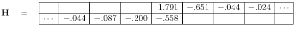
Although the autocorrelation $\bold r$ has mostly zero values, the factored autocorrelation $\bold a$ has a great number of nonzero terms. Fortunately, the coefficients seem to be shrinking rapidly towards a gap in the middle, so truncation (of those middle coefficients) seems reasonable. I wish I could show you a larger matrix, but all I can do is to pack the signal $\bold a$ into shifted columns of a lower triangular matrix $\bold A$ like this:

$$\bold A \ = \ \ \left[ \begin{array}{rrrrrrrrrrrr} 1.8& \cdot& \c... ...cdot& \cdot& \cdot& \cdot& \cdot& -.6& -.2&\ddots& -.6& 1.8 \end{array} \right]$$ (15)

If you allow me some truncation approximations, I now claim that the Laplacian represented by the matrix in equation (14) is factored into two parts $-\nabla^2 =\bold A\T\bold A$ , which are upper and lower triangular matrices whose product forms the autocorrelation seen in equation (14). Recall that triangular matrices allow quick solutions of simultaneous equations by backsubstitution, which is what we are doing with our deconvolution program.

Spectral factorization produces not merely a causal wavelet with the required autocorrelation. It produces one that is stable in deconvolution. Using $\bold H$ in 1-dimensional polynomial division, we can solve many formerly difficult problems very rapidly. Consider the Laplace equation with sources (Poisson's equation). Polynomial division and its reverse (adjoint) gives us $\bold p =(\bold q/\bold H)/\bold H\T$ , which means we have solved $\nabla^2 \bold p = -\bold q$ by using polynomial division on a helix. Using the 7 coefficients shown, the cost is 14 multiplications (because we need to run both ways) per mesh point. An example is shown in Figure 10.

lapfac
Figure 10. Deconvolution by a filter with autocorrelation being the 2-dimensional Laplacian operator. Amounts to solving the Poisson equation. Left is $\bold q$ ; Middle is $\bold q/\bold H$ ; Right is $(\bold q/\bold H)/\bold H\T$ .

Figure contains both the helix derivative and its inverse. Contrast those filters to the $x$ - or $y$ -derivatives (doublets) and their inverses (axis-parallel lines in the $(x,y)$ -plane). Simple derivatives are highly directional, whereas, the helix derivative is only slightly directional achieving its meagre directionality entirely from its phase spectrum.

The helical coordinate