|
|
|
|
The helical coordinate |
|
|---|
|
helocut
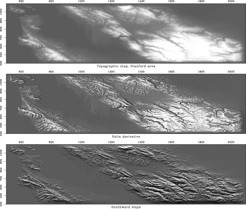
Figure 11. Topography, helical derivative, slope south. |
|
|
The operator ![]() has
curious similarities and differences
with the familiar gradient and divergence operators.
In 2-dimensional physical space,
the gradient maps one field to two fields
(north slope and east slope).
The factorization of
has
curious similarities and differences
with the familiar gradient and divergence operators.
In 2-dimensional physical space,
the gradient maps one field to two fields
(north slope and east slope).
The factorization of ![]() with the helix
gives us the operator
with the helix
gives us the operator ![]() that maps one field to one field.
Being a one-to-one transformation
(unlike gradient and divergence),
the operator
that maps one field to one field.
Being a one-to-one transformation
(unlike gradient and divergence),
the operator ![]() is potentially invertible
by deconvolution (recursive filtering).
is potentially invertible
by deconvolution (recursive filtering).
I have chosen the name
``helix derivative''
or ``helical derivative'' for the operator ![]() .
A flag pole has a narrow shadow behind it.
The helix integral (middle frame of Figure
.
A flag pole has a narrow shadow behind it.
The helix integral (middle frame of Figure ![]() )
and the helix derivative (left frame)
show shadows with an angular bandwidth approaching
)
and the helix derivative (left frame)
show shadows with an angular bandwidth approaching ![]() .
.
Our construction makes ![]() have the energy spectrum
have the energy spectrum
![]() ,
so the magnitude of the Fourier transform is
,
so the magnitude of the Fourier transform is
![]() .
It is a cone
centered at the origin with there the value zero.
By contrast, the components of the ordinary gradient
have amplitude responses
.
It is a cone
centered at the origin with there the value zero.
By contrast, the components of the ordinary gradient
have amplitude responses ![]() and
and ![]() that are lines of zero across the
that are lines of zero across the
![]() -plane.
-plane.
The rotationally invariant cone in the Fourier domain
contrasts sharply with the nonrotationally invariant
helix derivative in ![]() -space.
The difference must arise from the phase spectrum.
The factorization (13)
is nonunique because causality
associated with the helix mapping
can be defined along either
-space.
The difference must arise from the phase spectrum.
The factorization (13)
is nonunique because causality
associated with the helix mapping
can be defined along either ![]() - or
- or ![]() -axes;
thus the operator
(13)
can be rotated or reflected.
-axes;
thus the operator
(13)
can be rotated or reflected.
In practice, we often require an isotropic filter.
Such a filter is a function of
![]() .
It could be represented as a sum of helix derivatives to integer powers.
.
It could be represented as a sum of helix derivatives to integer powers.
If you want to see some tracks on the side of a hill,
you want to subtract the hill and see only the tracks.
Usually, however, you do not have a very good model for the hill.
As an
expedient, you could apply a low-cut filter to remove all
slowly variable functions of altitude.
In Chapter ![]() we found the Sea of Galilee
in Figure
we found the Sea of Galilee
in Figure ![]() to be too smooth for viewing pleasure,
so we made the roughened versions
in Figure
to be too smooth for viewing pleasure,
so we made the roughened versions
in Figure ![]() ,
a 1-dimensional filter that we could apply
over the
,
a 1-dimensional filter that we could apply
over the ![]() -axis or the
-axis or the ![]() -axis.
In Fourier space, such a filter has a response function of
-axis.
In Fourier space, such a filter has a response function of ![]() or a function of
or a function of ![]() .
The isotropy of physical space tells us
it would be more logical to design a filter that
is a function of
.
The isotropy of physical space tells us
it would be more logical to design a filter that
is a function of
![]() .
In Figure 11 we saw that the helix derivative
.
In Figure 11 we saw that the helix derivative
![]() does a nice job.
The Fourier magnitude of its impulse response is
does a nice job.
The Fourier magnitude of its impulse response is
![]() .
There is a little anisotropy connected with phase (which way should
we wind the helix, on
.
There is a little anisotropy connected with phase (which way should
we wind the helix, on ![]() or
or ![]() ?), but it is
not nearly so severe as that of either component of the gradient,
the two components having wholly different spectra,
amplitude
?), but it is
not nearly so severe as that of either component of the gradient,
the two components having wholly different spectra,
amplitude ![]() or
or ![]() .
.
|
|
|
|
The helical coordinate |