Time-shift imaging condition in seismic migration

Discussion

As discussed in one of the preceding sections, time-shift gathers consist of linear events with slopes corresponding to the local migration velocity. In contrast, space-shift gathers consist of events focused at ${ \bf h}=0$. Those events can be mapped to the angle-domain using transformations (20) and (23), respectively.

In order to understand the angle-domain mapping, we consider a simple synthetic in which we model common-image gathers corresponding to incidence at a particular angle. The experiment is depicted in Figure 15 for time-shift imaging, and in Figure 16 for space-shift imaging. For this experiment, the sampling parameters are the following: $\Delta z=0.01$ km, $\Delta h=0.02$ km, and $\Delta \tau=0.01$ s.

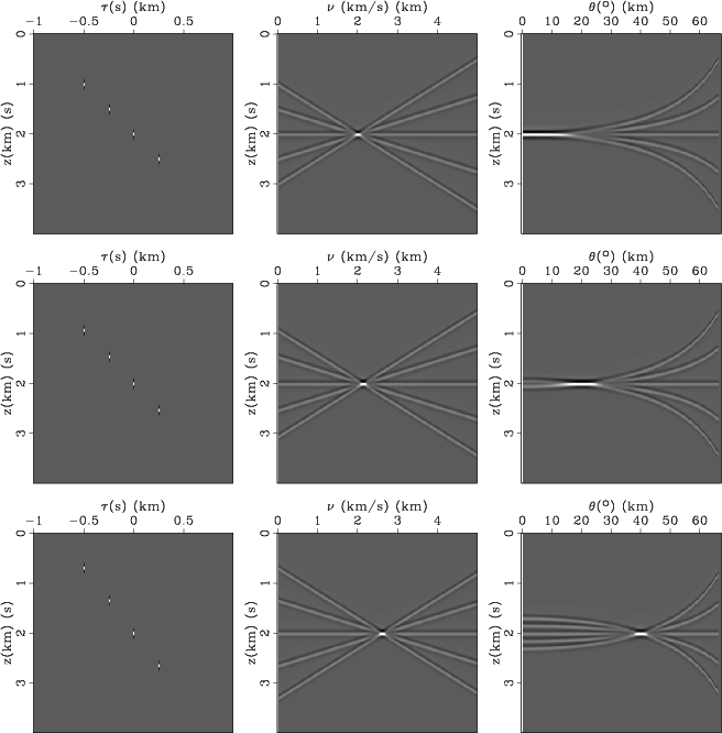
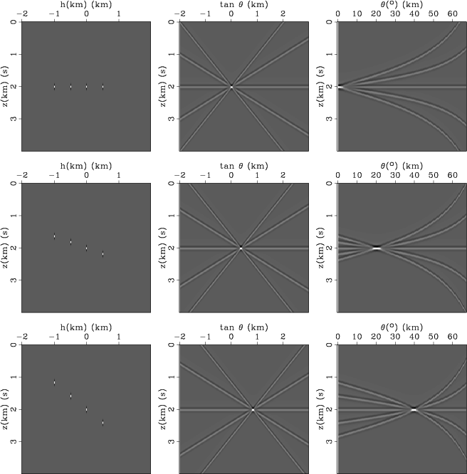
A reflection event at a single angle of incidence maps in common-image gathers as a line of a given slope. The left panels in Figures 15 and 16 show $3$ cases, corresponding to angles of $0 ^\circ$, $20^\circ$ and $40^\circ$. Since we want to analyze how such events map to angle, we subsample each line to $5$ selected samples lining-up at the correct slope.

The middle panels in Figures 15 and 16 show the data in the left panels after slant-stacking in $z-{ \tau}$ or $z-h$ panels, respectively. Each individual sample from the common-image gathers maps in a line of a different slope intersecting in a point. For example, normal incidence in a time-shift gather maps at the migration velocity $\nu=2$ km/s (Figure 15 top row, middle panel), and normal incidence in a space-shift gather maps at slant-stack parameter $\tan \theta =0$.

The right panels in Figures 15 and 16 show the data from the middle panels after mapping to angle using equations (23) and (20), respectively. All lines from the slant-stack panels map into curves that intersect at the angle of incidence.

We note that all curves for the time-shift angle-gathers have zero curvature at normal incidence. Therefore, the resolution of the time-shift mapping around normal incidence is lower than the corresponding space-shift resolution. However, the storage and computational cost of time-shift imaging is smaller than the cost of equivalent space-shift imaging. The choice of the appropriate imaging condition depends on the imaging objective and on the trade-off between the cost and the desired resolution.

ttest
Figure 15. Image-gather formation using time-shift imaging. Each row depicts an event at $0 ^\circ$ (top), $20^\circ$ (middle), and $40^\circ$ (bottom). Three columns correspond to subsampled time-shift gathers (left), slant-stacked gathers (middle), and angle-gathers (right).

htest
Figure 16. Image-gather formation using space-shift imaging. Each row depicts an event at $0 ^\circ$ (top), $20^\circ$ (middle), and $40^\circ$ (bottom). Three columns correspond to subsampled space-shift gathers (left), slant-stacked gathers (middle), and angle-gathers (right).

Time-shift imaging condition in seismic migration