|
|
|
|
Time-shift imaging condition in seismic migration |
|
|---|
|
IMGSLO0t
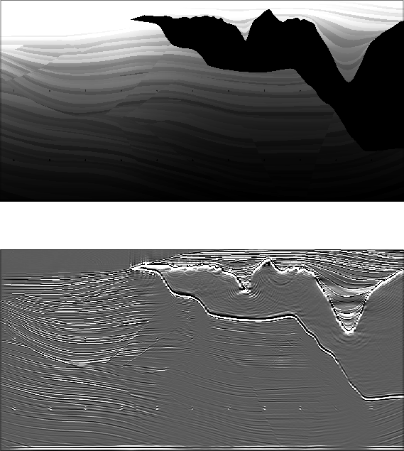
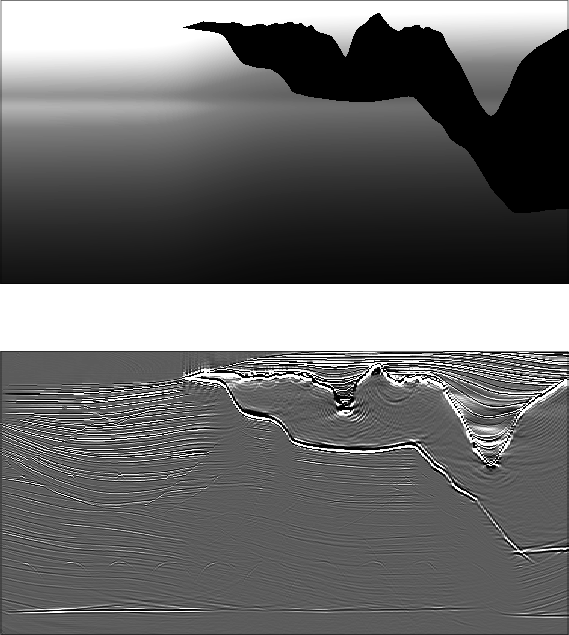
Figure 7. Sigsbee 2A model: correct velocity (top) and migrated image obtained by shot-record wavefield extrapolation migration with time-shift imaging condition (bottom). |
|
|
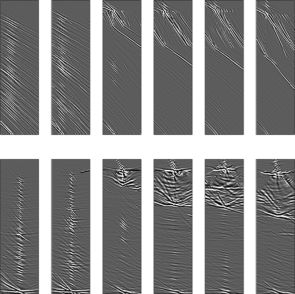
The top row of Figure 8 shows common-image gathers at
locations
![]() km
obtained by time-shift imaging condition.
As in the preceding synthetic
example, we can observe events with linear trends at slopes
corresponding to local migration velocity.
Since the migration velocity is correct, the strongest
events in common-image gathers correspond to
km
obtained by time-shift imaging condition.
As in the preceding synthetic
example, we can observe events with linear trends at slopes
corresponding to local migration velocity.
Since the migration velocity is correct, the strongest
events in common-image gathers correspond to ![]() .
For comparison,
the bottom row of Figure 8 shows
common-image gathers at the same locations
obtained by space-shift imaging condition.
In the later case, the strongest events occur at
.
For comparison,
the bottom row of Figure 8 shows
common-image gathers at the same locations
obtained by space-shift imaging condition.
In the later case, the strongest events occur at ![]() .
The zero-offset images (
.
The zero-offset images (![]() and
and ![]() ) are identical.
) are identical.
|
|---|
|
alloff
Figure 8. Imaging gathers at positions |
|
|
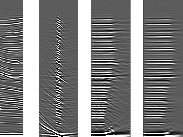
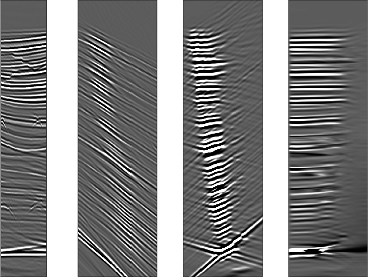
Figure 9 shows the angle-decomposition
for the common-image gather at location ![]() km.
From left to right, the panels depict
the migrated image,
a common-image gather resulting from
migration by wavefield extrapolation with time-shift imaging,
the common-image gather after slant-stacking
in the
km.
From left to right, the panels depict
the migrated image,
a common-image gather resulting from
migration by wavefield extrapolation with time-shift imaging,
the common-image gather after slant-stacking
in the ![]() plane, and an angle-gather
derived from the slant-stacked panel using equation equation (23).
plane, and an angle-gather
derived from the slant-stacked panel using equation equation (23).
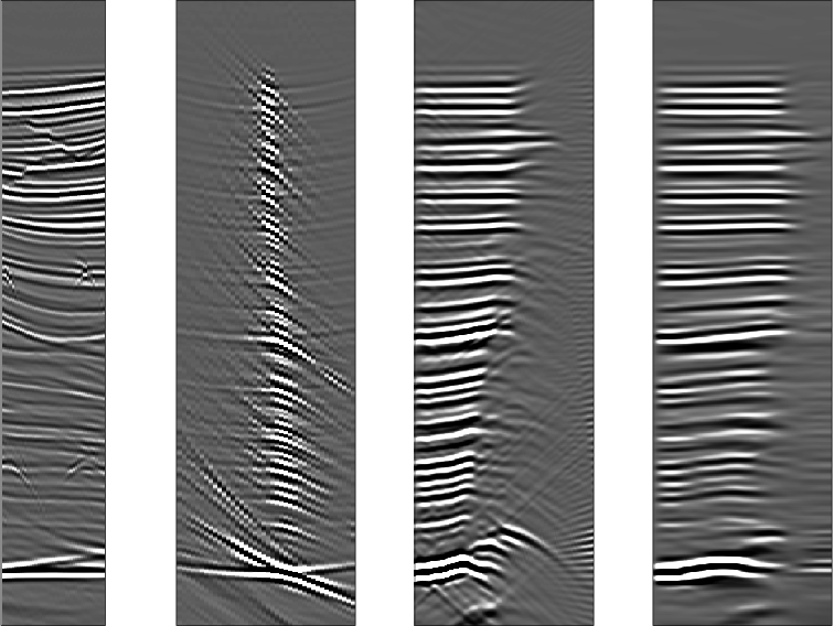
For comparison, Figure 10 depicts a similar process for a common-image gather at the same location obtained by space-shift imaging. Despite the fact that the offset gathers are completely different, the angle-gathers are comparable showing similar trends of angle-dependent reflectivity.

|
|---|
|
SRt0-7
Figure 9. Time-shift imaging condition gather at |
|
|
|
|---|
|
SRx0-7
Figure 10. Space-shift imaging condition gather at |
|
|
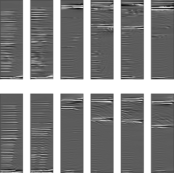
The top row of Figure 11 shows angle-domain
common-image gathers for time-shift imaging
at locations
![]() km.
Since the migration velocity is correct, all events are mostly
flat indicating correct imaging.
For comparison,
the bottom row of Figure 11 shows
angle-domain common-image gathers for space-shift
imaging condition at the same locations in the image.
km.
Since the migration velocity is correct, all events are mostly
flat indicating correct imaging.
For comparison,
the bottom row of Figure 11 shows
angle-domain common-image gathers for space-shift
imaging condition at the same locations in the image.
|
|---|
|
allang
Figure 11. Angle-gathers at positions |
|
|
Finally, we illustrate the behavior of
time-shift imaging with incorrect velocity.
The top panel in Figure 12 shows an incorrect
velocity model used to image the Sigsbee 2A data, and
the bottom panel shows the resulting image. The incorrect
velocity is a smooth version of the correct interval velocity,
scaled by ![]() from a depth
from a depth ![]() km downward.
The uncollapsed diffractors at depth
km downward.
The uncollapsed diffractors at depth ![]() km clearly indicate
velocity inaccuracy.
km clearly indicate
velocity inaccuracy.
|
|---|
|
IMGSLO2t
Figure 12. Sigsbee 2A model: incorrect velocity (top) and migrated image obtained by shot-record wavefield extrapolation migration with time-shift imaging condition. Compare with Figure 7. |
|
|
Figures 13 and 14 show
imaging gathers and the derived angle-gathers for time-shift and
space-shift imaging at the same location ![]() km.
Due to incorrect velocity, focusing does not occur
at
km.
Due to incorrect velocity, focusing does not occur
at ![]() or
or ![]() as in the preceding case.
Likewise, the reflections in angle-gathers are non-flat,
indicating velocity inaccuracies.
Compare Figures 9 and 13,
and Figures 10 and 14.
Those moveouts can be exploited for migration velocity
analysis
(Clapp et al., 2004; Sava and Biondi, 2004b,a; Biondi and Sava, 1999).
as in the preceding case.
Likewise, the reflections in angle-gathers are non-flat,
indicating velocity inaccuracies.
Compare Figures 9 and 13,
and Figures 10 and 14.
Those moveouts can be exploited for migration velocity
analysis
(Clapp et al., 2004; Sava and Biondi, 2004b,a; Biondi and Sava, 1999).
|
|---|
|
SRt2-7
Figure 13. Time-shift imaging condition gather at |
|
|
|
|---|
|
SRx2-7
Figure 14. Space-shift imaging condition gather at |
|
|
|
|
|
|
Time-shift imaging condition in seismic migration |