Next: Hankel tail
Up: Waves and Fourier sums
Previous: Passive seismology
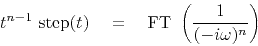
Causal integration
is represented in the time domain
by convolution with a step function.
In the frequency domain this amounts to multiplication by  .
(There is also delta function behavior at
.
(There is also delta function behavior at  which may be ignored in practice and since
at , wave theory reduces to potential theory).
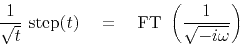
Integrating twice amounts to convolution by a ramp function,
which may be ignored in practice and since
at , wave theory reduces to potential theory).
Integrating twice amounts to convolution by a ramp function,
 , which in the Fourier domain is multiplication by
 .
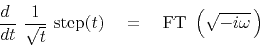
Integrating a third time is convolution with
.
Integrating a third time is convolution with
 which in the Fourier domain is multiplication by
 .
In general
.
In general
 |
(28) |
Proof of the validity of equation (28) for integer values of  is by repeated indefinite integration which also indicates
the need of an
is by repeated indefinite integration which also indicates
the need of an  scaling factor.
Proof of the validity of equation (28) for fractional values of
would take us far afield mathematically.
Fractional values of , however,
are exactly what we need to interpret Huygen's secondary wave sources in 2-D.
The factorial function of in the scaling factor becomes a gamma function.
The poles suggest that a more thorough mathematical study of convergence
is warranted, but this is not the place for it.
scaling factor.
Proof of the validity of equation (28) for fractional values of
would take us far afield mathematically.
Fractional values of , however,
are exactly what we need to interpret Huygen's secondary wave sources in 2-D.
The factorial function of in the scaling factor becomes a gamma function.
The poles suggest that a more thorough mathematical study of convergence
is warranted, but this is not the place for it.
The principal artifact
of the hyperbola-sum method of 2-D migration is the waveform
represented by equation (28) when  .
For , ignoring the scale factor,
equation (28) becomes
.
For , ignoring the scale factor,
equation (28) becomes
 |
(29) |
A waveform that should come out to be an impulse
actually comes out to be equation (29) because Kirchhoff
migration needs a little more than summing or spreading on a hyperbola.
To compensate for the erroneous filter response of equation (29)
we need its inverse filter.
We need
 .
To see what
is in the time domain,
we first recall that
.
To see what
is in the time domain,
we first recall that
 |
(30) |
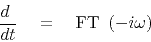
A product in the frequency domain corresponds
to a convolution in the time domain.
A time derivative is like convolution with a doublet
 .
Thus, from
equation (29) and
equation (30)
we obtain
.
Thus, from
equation (29) and
equation (30)
we obtain
 |
(31) |
Thus, we will see the way to overcome
the principal artifact of hyperbola summation
is to apply the filter of equation (31).
In chapter ![[*]](icons/crossref.png) we will learn more exact methods of migration.
There we will observe that an impulse in the earth
creates not a hyperbola with an impulsive waveform
but in two dimensions,
a hyperbola with the waveform of
equation (31),
and in three dimensions,
a hyperbola of revolution (umbrella?)
carrying a time-derivative waveform.
we will learn more exact methods of migration.
There we will observe that an impulse in the earth
creates not a hyperbola with an impulsive waveform
but in two dimensions,
a hyperbola with the waveform of
equation (31),
and in three dimensions,
a hyperbola of revolution (umbrella?)
carrying a time-derivative waveform.
Subsections
Next: Hankel tail
Up: Waves and Fourier sums
Previous: Passive seismology
2013-01-06