|
|
|
|
CuQ-RTM: A CUDA-based code package for stable and efficient Q-compensated reverse time migration |
Next: Module Up: Architecture of the cu-RTM Previous: Memory manipulation
|
|
|
|
CuQ-RTM: A CUDA-based code package for stable and efficient Q-compensated reverse time migration |
Kernels, the most basic unit of cu![]() -RTM to accomplish a series of specific tasks such as variable initialization and applying an absorbing boundary condition (ABC), can further be integrated into a fully functional module. Different variables are initialized with distinct kernels cuda_kernel_initialization(
-RTM to accomplish a series of specific tasks such as variable initialization and applying an absorbing boundary condition (ABC), can further be integrated into a fully functional module. Different variables are initialized with distinct kernels cuda_kernel_initialization(![]() ), cuda_kernel_initialization_images(
), cuda_kernel_initialization_images(![]() ), and cuda_kernel_initialization_Finals(
), and cuda_kernel_initialization_Finals(![]() ) based on their scope in modules. Wavefield variables are updated by cuda_kernel_update(
) based on their scope in modules. Wavefield variables are updated by cuda_kernel_update(![]() ).
).
In the framework of cu![]() -RTM, the basic forward and backward modules based on viscoacoustic wave equation with DFLs are efficiently simulated by PSM coupled with the CUFFT library. However, CUFFT library functions can only be executed on the device and called from the host, so we split the customized kernel functions into a k-space component and x-space component. The Fourier transform function cufftExecC2C(
-RTM, the basic forward and backward modules based on viscoacoustic wave equation with DFLs are efficiently simulated by PSM coupled with the CUFFT library. However, CUFFT library functions can only be executed on the device and called from the host, so we split the customized kernel functions into a k-space component and x-space component. The Fourier transform function cufftExecC2C(![]() , CUFFT_FORWARD) and inverse Fourier transform function cufftExecC2C(
, CUFFT_FORWARD) and inverse Fourier transform function cufftExecC2C(![]() , CUFFT_INVERSE) serve as the link between the x-space operator cuda_kernel_visco_PSM_2d_forward_x_space(
, CUFFT_INVERSE) serve as the link between the x-space operator cuda_kernel_visco_PSM_2d_forward_x_space(![]() ) and the k-space operator cuda_kernel_visco_PSM_2d_forward_k_space(
) and the k-space operator cuda_kernel_visco_PSM_2d_forward_k_space(![]() ). Absorbing boundary conditions for these modeling operators are conducted by the multiple transmitting formula (MTF) cuda_kernel_MTF_2nd(
). Absorbing boundary conditions for these modeling operators are conducted by the multiple transmitting formula (MTF) cuda_kernel_MTF_2nd(![]() ) (Liao et al., 1984).
) (Liao et al., 1984).
In the cu![]() -RTM package, we adopt the CATRC scheme to reconstruct source wavefields, which combines the efficiency of reverse propagation and the stability of checkpointing. Kernel functions cuda_kernel_checkpoints_Out(
-RTM package, we adopt the CATRC scheme to reconstruct source wavefields, which combines the efficiency of reverse propagation and the stability of checkpointing. Kernel functions cuda_kernel_checkpoints_Out(![]() ) and cuda_kernel_checkpoints_In(
) and cuda_kernel_checkpoints_In(![]() ) are designed to record and fetch forward wavefields at predefined checkpoints. Furthermore, wavefields on the outermost layer boundary of simulation domain at each time step are also recorded in global device variables
) are designed to record and fetch forward wavefields at predefined checkpoints. Furthermore, wavefields on the outermost layer boundary of simulation domain at each time step are also recorded in global device variables
![]() , and
, and
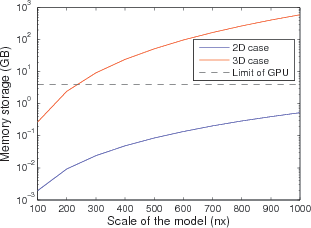
![]() . The total memory storage for 2D reconstruction can be estimated as
. The total memory storage for 2D reconstruction can be estimated as
|
|---|
|
Fig2a_v,Fig2b_v
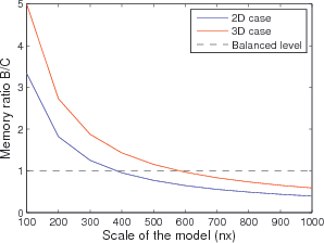
Figure 2. (a) Memory storage and (b) memory ratio of boundary wavefield to checkpointing wavefield (B/C) for both 2D and 3D cases. |
|
|
I develop an adaptive stabilization method to deal with numerical instability in ![]() -RTM, which exhibits superior properties of time-variance and
-RTM, which exhibits superior properties of time-variance and ![]() -dependence over conventional low-pass filtering. Both the adaptive stabilization scheme cuda_kernel_AdaSta(
-dependence over conventional low-pass filtering. Both the adaptive stabilization scheme cuda_kernel_AdaSta(![]() ) and low-pass filtering scheme cuda_kernel_filter2d(
) and low-pass filtering scheme cuda_kernel_filter2d(![]() ) are provided in this package. Users can choose either of these two stabilizing methods to suppress high-frequency noises as they like.
) are provided in this package. Users can choose either of these two stabilizing methods to suppress high-frequency noises as they like.
|
|
|
|
CuQ-RTM: A CUDA-based code package for stable and efficient Q-compensated reverse time migration |
![$\displaystyle Storage_{2D} [GB] \approx \frac{2(nx+nz) nt + (N_c+2) (nx \times nz)}{1024^3/4},$](img72.png)
![$\displaystyle Storage_{3D} [GB] \approx \frac{2(nx \times ny + nx \times nz + ny \times nz) nt + (N_c+2) (nx \times ny \times nz)}{1024^3/4},$](img73.png)