|
|
|
|
CuQ-RTM: A CUDA-based code package for stable and efficient Q-compensated reverse time migration |
Next: Discussion Up: Examples Previous: -RTM on Marmousi model
|
|
|
|
CuQ-RTM: A CUDA-based code package for stable and efficient Q-compensated reverse time migration |
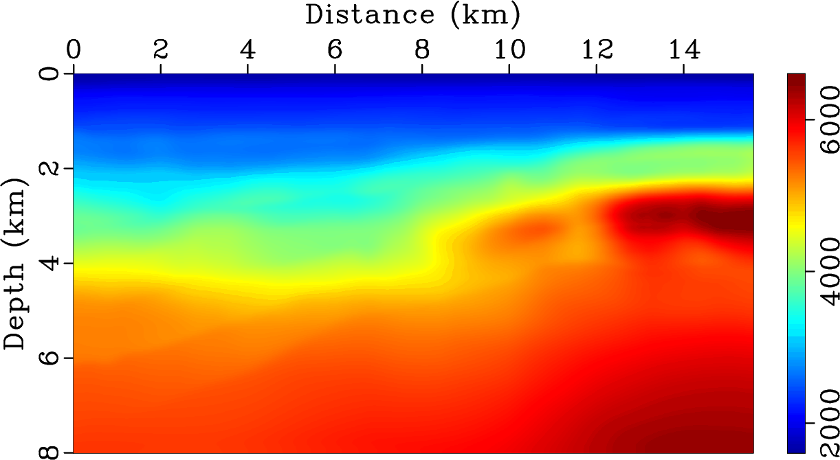
The field data example shown in Figures 9-11 aims to further verify the feasibility and applicability of the proposed package. Velocity and ![]() models are presented in Figure 9, which were obtained by migration velocity analysis (Sava and Vlad, 2008) and
models are presented in Figure 9, which were obtained by migration velocity analysis (Sava and Vlad, 2008) and ![]() tomography (Shen and Zhu, 2015). The size of the model is 8.0 km
tomography (Shen and Zhu, 2015). The size of the model is 8.0 km ![]() 15.6 km with the spatial interval
15.6 km with the spatial interval
![]() m. There are 77 shots horizontally distributed on the surface of the model. We perform
m. There are 77 shots horizontally distributed on the surface of the model. We perform
![]() time steps for each shot with the temporal interval
time steps for each shot with the temporal interval
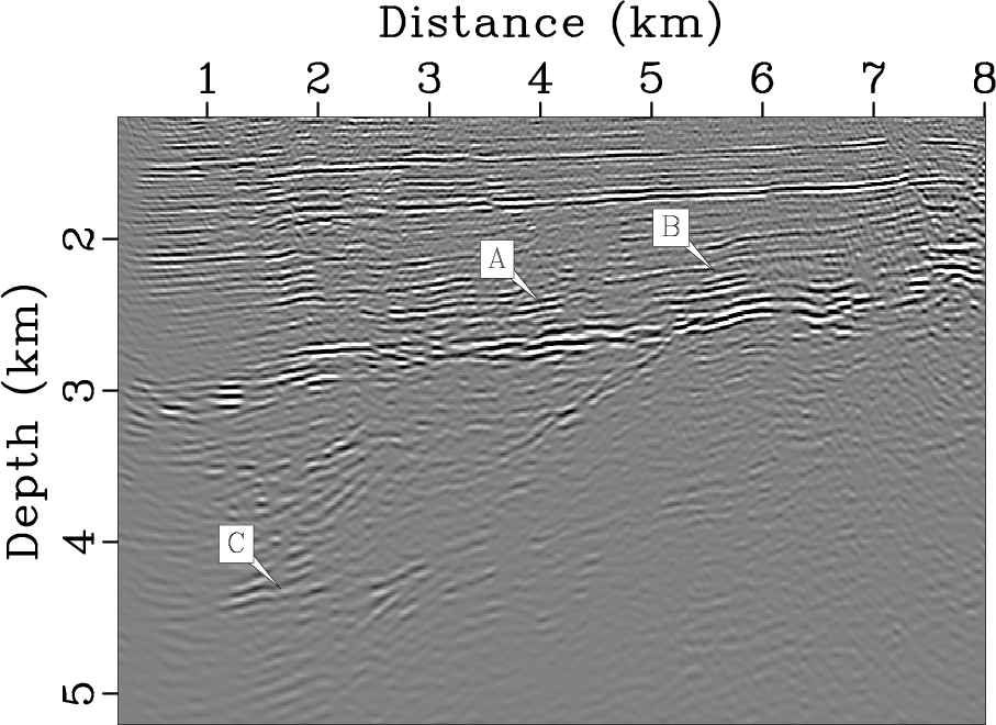
![]() s. In order to eliminate the diffraction artifacts from long offset, we set the stacking aperture of 2.0 km around the shot. Figure 10 shows the migrated image using conventional RTM without compensation (Figure 10a) and
s. In order to eliminate the diffraction artifacts from long offset, we set the stacking aperture of 2.0 km around the shot. Figure 10 shows the migrated image using conventional RTM without compensation (Figure 10a) and ![]() -RTM from real data (Figure 10b), respectively. For a clearer comparison, we display the zoomed in seismic images in Figure 11 corresponding to the marked area from Figure 10. From Figures 10a and 10b, one can conclude that the
-RTM from real data (Figure 10b), respectively. For a clearer comparison, we display the zoomed in seismic images in Figure 11 corresponding to the marked area from Figure 10. From Figures 10a and 10b, one can conclude that the ![]() -compensated image using the proposed package exhibits sharper reflections and more balanced amplitude.
-compensated image using the proposed package exhibits sharper reflections and more balanced amplitude.

|
|---|
|
Fig9a_v,Fig9b_v
Figure 9. (a) Velocity and (b) |
|
|


|
|---|
|
Fig10a_v,Fig10b_v
Figure 10. Migrated images of the field data using (a) conventional RTM from viscoacoustic media without compensation, (b) |
|
|

|
|---|
|
Fig11a_v,Fig11b_v
Figure 11. Zoom view of the images shown in the boxs in (a) Figure 10a and (b) Figure 10b. |
|
|
|
|
|
|
CuQ-RTM: A CUDA-based code package for stable and efficient Q-compensated reverse time migration |