|
|
|
|
Multi-channel quality factor Q estimation |
Next: Conclusions Up: Chen, 2019: Multi-channel Q Previous: Examples
|
|
|
|
Multi-channel quality factor Q estimation |
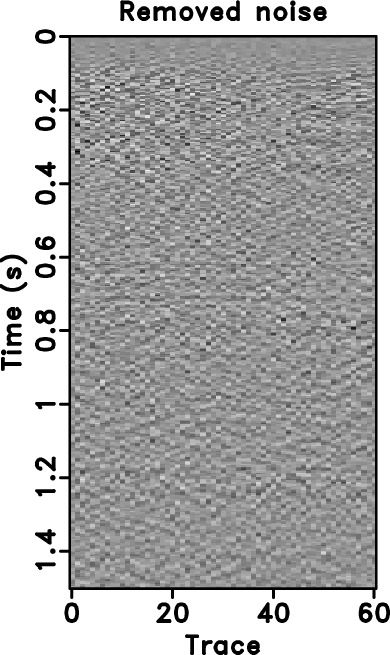
Although robust in the presence of strong noise, as can be concluded from the field data example, it is still instructive to see how the result from the proposed method is compared with the result from denoised data in a single-channel framework. Comparing the denoising-based traditional processing framework and the denoising-free multi-channel Q estimation framework can also be informative to evaluate the reliability of the new algorithm. For the raw field data shown in Figure 11a, we use the state-of-the-art ![]() predictive filtering (or FX Decon) method (Canales, 1984) to remove the noise first. The denoised data is shown in Figure 16a. Figure 16b shows the removed noise from the raw data.
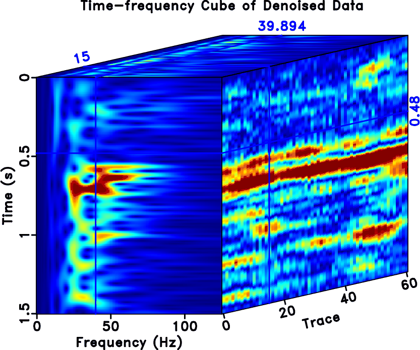
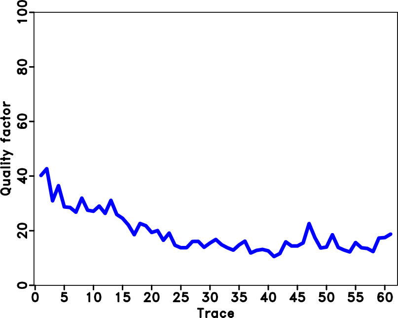
Comparing the denoised data in Figure 16a and the raw data in Figure 11a, it is clear to see the huge improvement. However, it is also possible to see some leaked signal energy, especially around the time slice of 0.6 s and 0.7 s. Figure 17 shows the time-frequency cube of the denoised field data. It is obvious that because of the removal of much random and coherent linear noise, the time-frequency cube of the denoised data becomes much clearer and smoother. Figure 18 shows the estimated Q from the denoised data using the single-channel method. The axes on Figure 18 are set the same as on Figure 15 for a easier comparison. From Figure 18 we observe that the estimated Q from the denoised data can be less oscillating compared with that from the raw data using the traditional single-channel framework. It indicates that the denoising step can indeed make the Q estimation more stable. However, the Q is still not continuous along the space direction and many abrupt changes in Q between neighbor channels still exist. It is surprising to see that the estimated Q from raw data using the new method and the estimated Q from denoised data using the traditional method are pretty close, indicating the fact that the new method can avoid a denoising step without much affecting the accuracy of the estimated Q.
predictive filtering (or FX Decon) method (Canales, 1984) to remove the noise first. The denoised data is shown in Figure 16a. Figure 16b shows the removed noise from the raw data.
Comparing the denoised data in Figure 16a and the raw data in Figure 11a, it is clear to see the huge improvement. However, it is also possible to see some leaked signal energy, especially around the time slice of 0.6 s and 0.7 s. Figure 17 shows the time-frequency cube of the denoised field data. It is obvious that because of the removal of much random and coherent linear noise, the time-frequency cube of the denoised data becomes much clearer and smoother. Figure 18 shows the estimated Q from the denoised data using the single-channel method. The axes on Figure 18 are set the same as on Figure 15 for a easier comparison. From Figure 18 we observe that the estimated Q from the denoised data can be less oscillating compared with that from the raw data using the traditional single-channel framework. It indicates that the denoising step can indeed make the Q estimation more stable. However, the Q is still not continuous along the space direction and many abrupt changes in Q between neighbor channels still exist. It is surprising to see that the estimated Q from raw data using the new method and the estimated Q from denoised data using the traditional method are pretty close, indicating the fact that the new method can avoid a denoising step without much affecting the accuracy of the estimated Q.

|
|---|
|
field-dn,field-dn-n
Figure 16. Denoising test. (a) Denoised field data using the |
|
|
|
|---|
|
field-dn-st-N
Figure 17. Time-frequency cube of the denoised field data. Note that the time-frequency map is much smoother than that from the raw data (Figure 12). |
|
|
|
|---|
|
field-dn-Q1s-esti
Figure 18. The estimated Q from the denoised data using the single-channel method. |
|
|
To understand the computational complexity of the proposed multi-channel Q estimation method, we need to analyse its implementation in detail. The main computational steps in the multi-channel Q estimation method are the forward S transform, regularization spectral division, and least-squares line-fitting. Let the target multi-channel seismic section be of the size ![]() . When transformed into the time-frequency domain, the 3D time-frequency cube is of the size
. When transformed into the time-frequency domain, the 3D time-frequency cube is of the size ![]() . The number of iterations during the regularized spectral division is
. The number of iterations during the regularized spectral division is ![]() , which is normally less than 50. The smoothing radii for the frequency and space directions are
, which is normally less than 50. The smoothing radii for the frequency and space directions are ![]() and
and ![]() , respectively. The computational cost of the typical forward S transform on the raw 2D seismic section is
, respectively. The computational cost of the typical forward S transform on the raw 2D seismic section is
![]() . With iterative solver, the inversion-based spectral division takes
. With iterative solver, the inversion-based spectral division takes
![]() , where the first term comes from the iterative conjugate gradient solver, and the latter two terms come from the smoothing regularization in the frequency and space directions. The least-squares line-fitting takes only
, where the first term comes from the iterative conjugate gradient solver, and the latter two terms come from the smoothing regularization in the frequency and space directions. The least-squares line-fitting takes only ![]() . Overall, since normally the computational cost of the regularized spectral division is much smaller than that of the S transform, the main computational cost of the proposed algorithm framework comes from the forward S transform. The traditional single-channel Q estimation method differs with the regularized one only in the second step, i.e., the inversion-based spectral division. In traditional single channel method, the cost is
. Overall, since normally the computational cost of the regularized spectral division is much smaller than that of the S transform, the main computational cost of the proposed algorithm framework comes from the forward S transform. The traditional single-channel Q estimation method differs with the regularized one only in the second step, i.e., the inversion-based spectral division. In traditional single channel method, the cost is ![]() . In the case of single-channel regularized spectral division, the cost is
. In the case of single-channel regularized spectral division, the cost is
![]() , which is only smaller than the proposed multi-channel method by
, which is only smaller than the proposed multi-channel method by
![]() . Considering that the smoothing radius in the proposed method is not chosen too large to avoid over-smoothing, the extra computational cost from the multi-channel method is not significant. In summary, the computational cost of the spectral ratio method is mainly from the S transform and improving the efficiency of the S transform is beneficial in increasing the efficiency of the overall algorithm framework.
. Considering that the smoothing radius in the proposed method is not chosen too large to avoid over-smoothing, the extra computational cost from the multi-channel method is not significant. In summary, the computational cost of the spectral ratio method is mainly from the S transform and improving the efficiency of the S transform is beneficial in increasing the efficiency of the overall algorithm framework.
|
|
|
|
Multi-channel quality factor Q estimation |