 |
 |
 |
 | From modeling to full waveform inversion: A hands-on tour using Madagascar |  |
![[pdf]](icons/pdf.png) |
Next: Reconstruct your source/incident wavefield
Up: From modeling to full
Previous: Further exercises
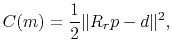
FWI is a nonlinear iterative minimization process by matching the waveform between the synthetic data and the observed seismograms (Virieux and Operto, 2009; Tarantola, 1984). In least-squares sense, the misfit functional of FWI reads
 |
(5) |
where  is the model parameter (i.e. the velocity) in model space;
  is a restriction operator mapping the wavefield onto the receiver locations;
 is the observed seismogram at receiver location
  while
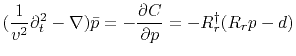
while  is the synthetic wavefield whose adjoint wavefield
  is given by
 |
(6) |
which indicates that the adjoint wave equation is exactly the same as the forward wave equation except that the adjoint source is data residual backprojected into the wavefield.
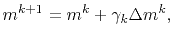
In each iteration the model has to be updated following a Newton descent direction

 |
(7) |
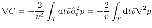
with a stepsize  . Away from the sources (
 ), the gradient can be computed by
 |
(8) |
Subsections
|
|
|
|
| From modeling to full waveform inversion: A hands-on tour using Madagascar | |
|
Next: Reconstruct your source/incident wavefield
Up: From modeling to full
Previous: Further exercises
2021-08-31