Fourier pseudo spectral method for attenuative simulation with fractional Laplacian

Computing derivatives using Fourier transform

The Fourier transform of a function $f(x)$ and the inverse are define respectively

$$\tilde{f}(\omega)=F[f]=\int f(x)e^{-i\omega x}\mathrm{d}x$$ (4)

and

$$f(x)=F^{-1}[f]=\frac{1}{2\pi}\int \tilde{f}(\omega)e^{i\omega x}\mathrm{d}\omega$$ (5)

where $\tilde{f}$ is the Fourier transform of $f$ . In spatial dimension, $\omega$ corresponds to the wavenumber $k$ . Therefore we have

$$\partial_x f=\partial_x\left( \frac{1}{2\pi}\int \tilde{f}e^{ik_x... ...{d}x\right) = \frac{1}{2\pi}\int \underline{ik_x\tilde{f}}e^{ik_x x}\mathrm{d}x$$ (6)

and

$$\partial_{xx} f=\partial_{xx}\left( \frac{1}{2\pi}\int \tilde{f}e... ...\right) = \frac{1}{2\pi}\int \underline{(ik_x)^2\tilde{f}}e^{ik_x x}\mathrm{d}x$$ (7)

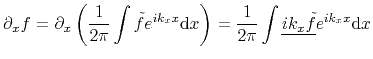
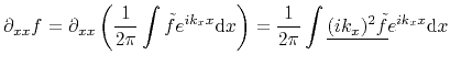
The term $\partial_x\left(\frac{1}{\rho}\partial_x p\right)$ will be calculated by the following precedure:

$$\begin{array}{rl} p\stackrel{F}{\longrightarrow}& \tilde{p}\\... ...{-1}[ik_xF[\frac{1}{\rho}F^{-1}[ik_x\tilde{p}]]] \\ \end{array}$$ (8)

Let us conduct a 2-D numerical simulation of acoustic wave equation with constant density. The equation is then

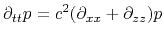$$\partial_{tt}p=c^2 (\partial_{xx}+\partial_{zz})p$$ (9)

Based upon Fourier transform for spatial axis, we know the right hand side of the above equation corresponds to

$$-(k_x^2+k_z^2)\tilde{p}$$ (10)

Thus, we have the following time evolution

$$p^{n+1}=2p^n-p^{n-1}+\Delta t^2 c^2F^{-1}[-(k_x^2+k_z^2)F p^n]$$ (11)

Fourier pseudo spectral method for attenuative simulation with fractional Laplacian