Fourier pseudo spectral method for attenuative simulation with fractional Laplacian

What is a pseudo-spectral method?

Spectral solutions to time-dependent PDEs are formulated in the frequency-wavenumber domain and solutions are obtained in terms of spectra (e.g. seismograms). This technique is particularly interesting for geometries where partial solutions in the $\omega-k$ domain can be obtained analytically (e.g. for layered models).

In the pseudo-spectral approach - in a finite-difference like manner - the PDEs are solved pointwise in physical space $(x-t)$ . However, the space derivatives are calculated using orthogonal functions (e.g. Fourier Integrals, Chebyshev polynomials). They are either evaluated using matrix-matrix multiplications, fast Fourier transform (FFT), or convolutions.

Let us start with the 1-D acoustic wave equation.

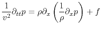$$\frac{1}{v^2}\partial_{tt}p=\rho\partial_x\left(\frac{1}{\rho}\partial_x p\right)+f$$ (1)

Omitting the source term, we may discretize the wave equation using standard centered finite difference for time stepping as

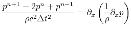$$\frac{p^{n+1}-2p^n+p^{n-1}}{\rho c^2\Delta t^2}=\partial_x\left(\frac{1}{\rho}\partial_x p\right)$$ (2)

where we use the notation 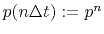$p(n\Delta t):=p^n$ . Thus, we have the following evolution scheme

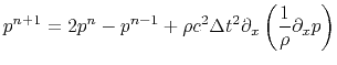$$p^{n+1}=2p^n-p^{n-1}+\rho c^2\Delta t^2 \partial_x\left(\frac{1}{\rho}\partial_x p\right)$$ (3)

where the space derivatives will be calculated using the Fourier transform.

Fourier pseudo spectral method for attenuative simulation with fractional Laplacian