|
|
|
|
IWAVE Structure and Basic Use Cases |
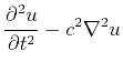 |
(1) | ||
 |
 |
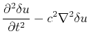
(2) |
As explained above, the IWAVE framework provides approximations for computing the linearization (widely called the ``Born approximation'', even though this is strictly a misnomer), along with its adjoint and higher derivatives.
The parameter key deriv flags the computation, or not, of
derivatives. The value assigned is the order of derivative, with
default 0. Each input perturbation (representing quantities such as
![]() in the linearized system of PDEs, above) is assigned a key
equal to the key for the unperturbed quantity with _d1 appended
(for the first derivative - higher derivatives require multiple input
perturbations, keys for which have _d2,
_d3,... appended). Output keys remain the same as for the reference
computation.
in the linearized system of PDEs, above) is assigned a key
equal to the key for the unperturbed quantity with _d1 appended
(for the first derivative - higher derivatives require multiple input
perturbations, keys for which have _d2,
_d3,... appended). Output keys remain the same as for the reference
computation.
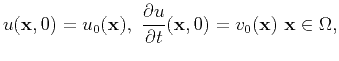
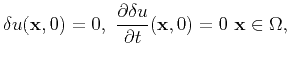
For the acoustic constant density application, Born approximation requires reference and perturbation square velocity fields. Figures 7 and 8 show perturbation and reference square velocity fields, respectively, that will generate Born data roughly corresponding to the preceding example. The required parameters are
         deriv = 1
           csq = ../csq_4layer.rsf
        csq_d1 = ../dcsq_4layer.rsf
        source = ../wavelet12000.su
          data = ../born12000.su
The linearized response (Born modeling) corresponding to Figure
6 appears as Figure 9.

|
|---|
|
dcsq-4layer
Figure 7. Velocity-squared perturbation - localized oscillations at layer boundaries |
|
|

|
|---|
|
csq-4layersm
Figure 8. Smooth velocity-squared obtained from velocity of Figure 1 by filtering with a cubic spline window. |
|
|

|
|---|
|
born12000
Figure 9. Linearized response (``Born modeling'') of seafloor pressure sensor, due to perturbation (Figure 7) about smooth background (Figure 8); other parameters as in Figure 6. |
|
|
|
|
|
|
IWAVE Structure and Basic Use Cases |